Wind regimes and their relation to synoptic variables using self-organizing maps

This study exemplifies the ability of the self-organizing maps (SOM) method to directly define well known wind regimes over Israel during the entire year, except summer period, at 12:00 UTC. This procedure may be applied at other hours and is highly relevant to future automatic climatological analysis and applications.

The investigation is performed by analysing surface wind measurements from 53 Israel Meteorological Service stations. The relation between the synoptic variables and the wind regimes is revealed from the averages of ECMWF ERA-INTERIM reanalysis variables for each SOM wind regime.

The inspection of wind regimes and their average geopotential anomalies has shown that wind regimes relate to the gradient of the pressure anomalies, rather than to the specific isobars pattern. Two main wind regimes – strong western and the strong eastern or northern – are well known over this region. The frequencies of the regimes according to seasons is verified. Strong eastern regimes are dominant during winter, while strong western regimes are frequent in all seasons.

1 Introduction

Winter (December, January, February – DJF) wind regimes over Israel by self-organizing maps (SOM) were previously defined (Berkovic, 2017). This study extends this ability to other seasons. Therefore, some of the sections of Berkovic (2017) are repeated here for clarity. The climate in Israel is a Mediterranean climate, with a hot and dry summer, transitional seasons and rainy winter. Since the summer regime is well known it was omitted from the study. During the summer there is a single synoptic group (Persian trough) with a typical wind regime exhibiting diurnal veering according to the diurnal heating and topography (Skibin and Hod, 1979; Ziv et al., 2004). During the winter and the transitional seasons synoptic variability increases and therefore, a higher number of surface wind regimes prevail. Many previous studies referred to a subjective or semi-objective synoptic classification (Alpert et al., 2004); however, there is a need for an automatic objective classification when studying the surface winds on an hourly time scale. An automatic algorithm will greatly facilitate the definition of wind regimes or synoptic classes, since a subjective analysis is highly tedious. This study shows the ability of SOM to automatically reconstruct previous subjective studies (Saaroni et al., 1998; Levy et al., 2008; Ziv and Yair, 1994; Goldreich, 2003) characterizing the surface flow over Israel.

SOM (self-organizing maps, Hewitson and Crane, 2002; Liu et al., 2006; Liu and Weisberg, 2011) is an objective non-linear clustering technique extensively used to determine the patterns of meteorological variables, e.g., sea surface temperature, wind, or geopotential height. This study employed SOM to define surface wind regimes over Israel at 12:00 UTC during winter, spring and autumn. The wind patterns are derived from surface wind measurements. Wind regimes at other synoptic hours (00:00, 06:00, 18:00 UTC) are not shown here for the sake of brevity. The relation between surface wind patterns and synoptic conditions is clarified by calculating the averages of the synoptic variables according to the SOM classification. The synoptic variables were derived from ECMWF ERA-INTERIM reanalysis data.

Section 2 describes the method and the data, Sect. 3 presents the SOM wind patterns and their relation to synoptic variables with references to previous works. Section 4 studies the frequencies of the wind regimes according to seasons and Sect. 5 concludes the study.

2 Data and methodology

The surface wind regimes were derived from 10 minute averages of surface wind measurements at 53 stations of the Israel Meteorological Service (IMS) from January 2006 to May 2012. The data was provided by the IMS. The measurements were performed 10 m above the ground by anemometers, mostly in rural areas. For each station there will be, in principle, 1880 events at each synoptic hour from the 9 months: December, January till May, September, October and November during January 2006–May 2012. The data were automatically monitored and registered as well as examined by a basic quality check. The authors further performed removal of outliers (> 30 m s⁻¹ based on experience and climatological statistics) and set low speed (< 0.5 m s⁻¹) events to be 0 m s⁻¹ wind speed and 0^∘ wind direction. Consistency between averages of wind speed and direction according to X:00 or X:10 events was found under each SOM regime.

The topography of the area and the location of the stations are presented in Fig. 1. The description given here has been adapted from the article by Skibin and Hod (1979). The Mediterranean coastal plain is relatively flat with its width varying from ∼ 50 km in the south of the map to ∼ 1 km near Haifa. Further north the width ranges from 2 to 12 km. Parallel to the coast, a mountain ridge with peaks 800–1200 m a.m.s.l. (above mean sea level) extends from north to south, interrupted by the Jezreel Valley East of Haifa. The mountains are the Judea and Samaria mountains to the south and the Galilee Mountains to the north. Further to the east, the Jordan valley runs parallel to the ridge, having a depth between 70 m below MSL in the north and to 400 m b.m.s.l. (below mean sea level) in the Dead Sea. The Jordan River flows from the Sea of Galilee to the Dead Sea. South of the Dead Sea lies the Arava valley. A second mountain ridge resides to the east of the Jordan River.

The IMS stations are situated in four major regions: (1) along the coast and the western slopes of the Judea and Samaria mountains. (2) Along the peak of the Judea and Samaria mountains. (3) The Galilee Mountains. (4) The Jordan and the Arava valleys including the Dead Sea area.

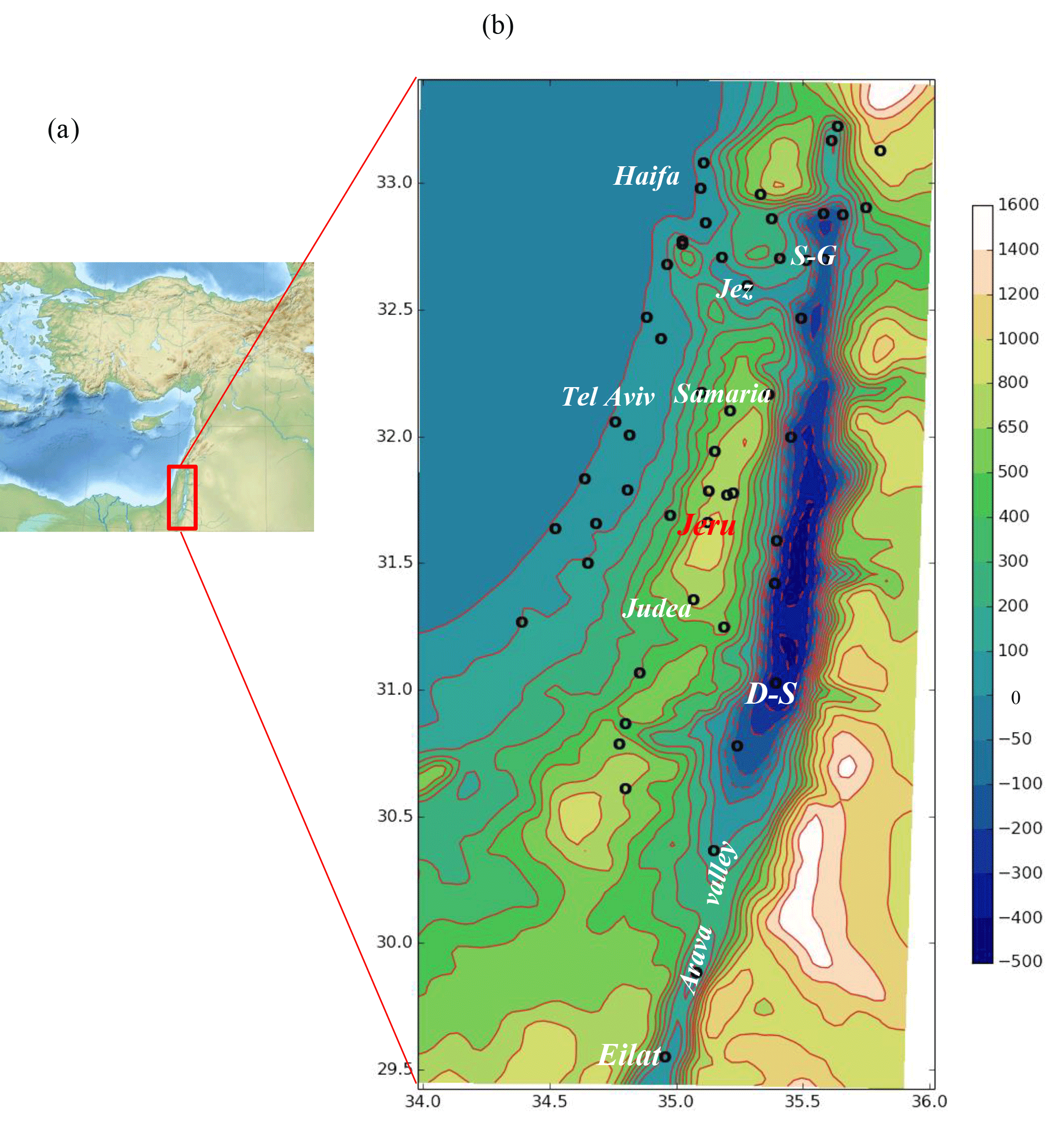
Figure 1 The East Mediterranean region (a) and the studied area (b) showing Jerusalem (Jeru), the Dead Sea (D-S), the Sea of Galilee (S-G), Jezreel valley (Jez). The locations of the 53 IMS stations are denoted by circles. The topography height above sea level [m] is denoted by colors and contour lines.

The average synoptic variables (temperature, specific humidity, zonal and meridional wind components, geopotential anomaly) at the chosen pressure levels: 1000, 925, 850, 500 hPa were calculated from ECMWF ERA-INTERIM data (Berrisford et al., 2011). ERA-INTERIM is a global atmospheric reanalysis from 1979, continuously updated in real time. It includes a 4-dimensional variational analysis (4D-Var) with a 12 h analysis window assimilating surface and upper air measurement data into the model. The spatial resolution of the reanalysis data is (1.25^∘) approximately 80 km (T255 spectral) on 60 vertical levels from the surface up to 0.1 hPa. The downloaded model horizontal resolution data was 0.75^∘. The time resolution of the data is 6 h.

SOM maps were calculated by the freely available SOM software package som-pak. A description of the software is provided by Kohonen et al. (1996). The SOM method uses an unsupervised and objective classification procedure to group events into clusters. The description and application of this method to surface winds was presented by Nigro and Cassano (2014). Each cluster is identified by a common pattern designated by a node. The patterns are displayed in a two dimensional array, that is known as a map of nodes (Kohonen, 2001). Unlike clustering methods, SOM does not need an initial guess of the clusters involved. The nodes present the dominant patterns ordered according to the time order presented in the data set. Similar nodes are located next to each other and contrasting nodes are further apart. Very different states map to the corners and edge of the map. More nodes are clustered according to their frequency in time across the data. Each node is an approximation to the mean of its members.

The software was applied to 10 min wind averages from winter, spring and autumn 2006–2012 from 53 IMS weather stations. The SOM was trained with the u- and v-components of the wind data. In order to characterize wind regimes at each synoptic hour, it is necessary to perform a separate study for each synoptic hour (Berkovic, 2017). In this approach, the diurnal time scale is omitted and it is possible to fully and independently resolve the wind regimes at each hour. Each synoptic hour should have 1880 days, but the data base had missing events. Only 1791 days were found in the database, on some days up to 30 % of the stations had missing data. The SOM PAK can handle missing data points (Kohonen et al., 1996; Samad and Harp, 1992). Allowing gappy input data is one of the many advantages of the SOM over other conventional methods (Liu and Weisberg, 2005). The SOM PAK routines compute the distance calculations and reference vector modification steps using the available data components. Samad and Harp (1992) have exemplified incomplete SOM training. When the probability of a missing datum was less than 0.6, the map entropy and RMSE were practically equal to those obtained from full data training.

SOM training is performed by an ordered examination of SOM maps. During this process the number of the nodes increases. The process ends when further increase of the number of nodes does not give new information. The map is a two dimensional rectangular array of nodes, the number of nodes in each map (map size) is denoted by N × M indicating the number of columns, N and the number of rows M, of the map. SOM nodes display patterns according to their frequency. Increasing the size of the map and keeping the size of the dataset will result in lower representativeness of the nodes.

The winter, spring and autumn surface winds at 12:00 UTC were separately studied. A series of 5 × 2, 7 × 2, 4 × 3, 5 × 3, 6 × 3 and 5 × 4 maps were created to determine the best map representing the variety of the wind patterns. Eventually the 4 × 3 map was selected at 12:00 UTC. The same method has been used for each of the remaining synoptic hours (00:00, 06:00, 18:00 UTC) data. It was found that 5 × 3 SOM map is representative at the remaining hours.

The determination of the wind regimes was followed by the calculation of the average wind field and steadiness at each node. This check ascertains that the SOM wind regime is similar to the average of its members, as expected (Nigro and Cassano, 2014). Since directionality is an important characteristic of the wind regime, an effort was made to choose the best SOM analysis which provides the highest degree of steadiness for most of the regimes according to the synoptic hour.

At each node, the average wind field and the wind steadiness were calculated (Berkovic, 2016). The steadiness parameter S is redefined here for clarity. The ratio of the mean wind vector M_V and the mean wind speed M_sp, is defined as follows:

$$\begin{array}{}\text{(1)}& {\displaystyle }& {\displaystyle }{M}_{\mathrm{V}}=\sqrt{{\left({\displaystyle \frac{\mathrm{1}}{N}}\sum _{i=\mathrm{1}}^N{u}_i\right)}^{\mathrm{2}}+{\left({\displaystyle \frac{\mathrm{1}}{N}}\sum _{i=\mathrm{1}}^N{v}_i\right)}^{\mathrm{2}}}\text{(2)}& {\displaystyle }& {\displaystyle }{M}_{\mathrm{sp}}={\displaystyle \frac{\mathrm{1}}{N}}\sum _{i=\mathrm{1}}^N\sqrt{u_i^{\mathrm{2}}+v_i^{\mathrm{2}}}\end{array}$$

$$\begin{array}{}\text{(3)}& {\displaystyle }{\displaystyle }S={\displaystyle \frac{M_{\mathrm{V}}}{M_{\mathrm{sp}}}}.\end{array}$$

S is equal to 1, when the wind flow is constant. When S < 0.5, the wind is not steady. According to a previous study (Berkovic, 2016), high S values were obtained when the standard deviation (SD) of the wind direction was relatively small (< 60^∘).

In order to study the relation between the synoptic parameters and the local wind regimes, the averages of the synoptic variables, derived from the ERA-INTERIM reanalysis data, were calculated at each node. Each average is an average over all the events classified for a certain wind regime. The effect of the synoptic pressure on the diurnal flow is studied by calculating the averages of the geopotential (ERA-Igp) height anomalies (Nigro and Cassano, 2014) for every wind pattern. The anomalies facilitate the comparison between the wind regimes at different hours since the effect of the average geopotentail (gp) height is removed. It is the pressure gradient which is responsible for the wind field, and not the absolute value of the gp height. The average ERA-Igp was calculated for a domain of 15 × 15 grid points around Israel between lat 27–38.25^∘ N and lon 29.25–40.5^∘ E. The anomaly was calculated by removing the area average at each time step. A very similar area was chosen by Alpert et al. (2004) to define the semi objective synoptic classes over the Eastern Mediterranean. Therefore, it is easy to relate to previous familiar semi objective synoptic classes. The typical pressure gradients according to the semi objective classification were presented in Berkovic (2016). The ERA-INTERIM temperature and humidity averages at each wind regime are presented over a smaller domain between 30.75–37.5^∘ E and 27–37^∘ N to inspect the temperature and specific humidity over Israel. Israel is covered by only six grid points between lon 34.5–35.25^∘ N and lat 33–30^∘ E.

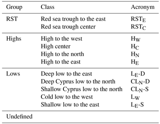
The East Mediterranean (EM) synoptic classes were mentioned in previous works (e.g., Alpert et al., 2004; Osetinsky, 2006; Berkovic, 2016). The frequent groups and classes are summarized in Table 1.

Table 1 The winter synoptic groups and classes.

3 Results

3.1 Winter, spring and autumn wind regimes at 12:00 UTC

A separate SOM analysis at 12:00 UTC during winter, spring and autumn was performed. Wind regimes at 12:00 UTC according to 4 × 3 SOM map will be presented and discussed. In all figures, the vectors display the average surface wind at each SOM node. S is denoted by circles according to size and color. The nodes are numbered sequentially from 1 to 12. The frequency (average number of events for all 53 stations) is displayed at the top of each sub figure. When presenting the average surface wind, around 1 % is lost due to weak winds (speed < 0.5 ms⁻¹). The weak wind events were included in the SOM analysis; however they were omitted from the calculation of wind averages in order to obtain the average wind direction under weak wind regimes. It is not possible to get an indicative wind direction for wind speed < 0.5 ms⁻¹.

From inspections of the SOM maps at all the synoptic hours, three dominant wind patterns are revealed:

1. western and southern wind which includes the strong (5–10 ms⁻¹) western flow over Israel;

2. eastern and northern flow which includes the strong (5–10 ms⁻¹) eastern flow to the north of Israel, and at the top of the Judea and Samaria mountain ridges;

3. relatively low speed (< 4 ms⁻¹) and directionality according to the diurnal heating and local topography or no directionality.

These main patterns of the wind regimes were previously found according to the winter analysis (Berkovic, 2017). A subjective classification by Saaroni et al. (1998), Levy et al. (2008), Goldreich (2003), Ziv and Yair (1994) links between the above 3 categories and the following semi-objective synoptic groups (Alpert et al., 2004; Dayan et al., 2012):

1. winter lows and highs from the west,

2. winter highs, Red Sea trough (RST),

3. shallow classes: high over Israel, shallow low from the west, shallow high from the west, shallow RST.

The wind regimes at 12:00 UTC will be hereon described according to the three dominant wind categories.

3.2 Surface wind regimes at 12:00 UTC

The wind patterns at 12:00 UTC are displayed in Fig. 2.

3.2.1 Category A: western wind

The strong (4–10 ms⁻¹) western wind regimes (nodes 2–4, Fig. 2) with high S (≥ 0.8) over Israel, except the Jordan and Arava valleys, relate to the location and pressure gradient of the winter lows (Ziv and Yair, 1994).

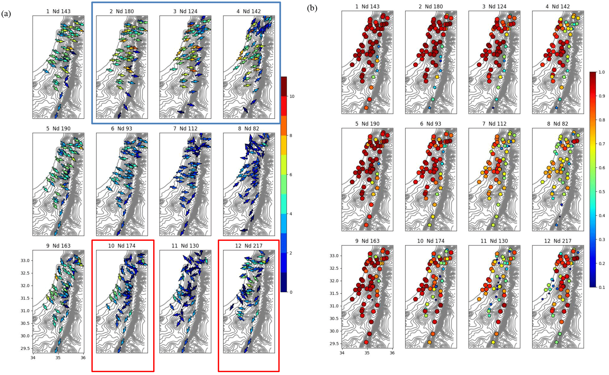
Figure 2 12:00 UTC winter, spring and autumn. (a) Average surface wind [m s⁻¹] patterns and (b) S-steadiness parameter. These values were calculated according to 4 × 3 SOM classification. The node number and the average (over the 53 stations) number of events, Nd, are shown at the top of each sub-figure. Red lines designate strong eastern wind regimes. Blue lines designate strong western wind regimes.

Figure 3 Number of occurrences for each node per month.

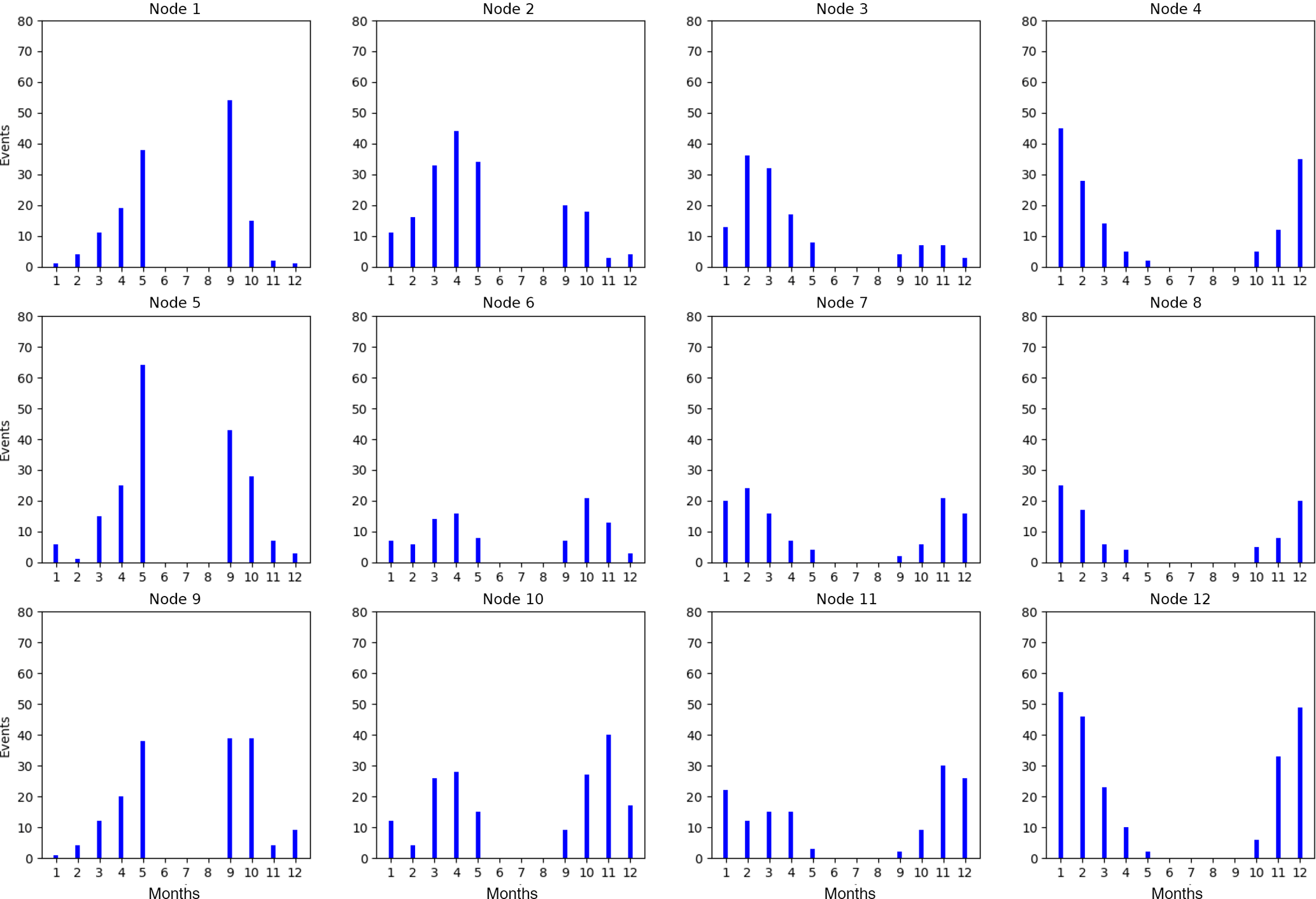
Figure 4 12:00 UTC winter spring and autumn, ERA-INTERIM averages according to 4 × 3 SOM wind regimes (displayed in Fig. 2). The node number is shown at the top of each sub-figure. (a) Average geopotential height anomalies over the EM [m² s⁻²] at 925 hPa. (b) Average temperature [^∘C] at 1000 hPa. (c) Average specific humidity [dg kg⁻¹] at 925 hPa. (d) Average synoptic wind [m s⁻¹] at 1000 hPa.

3.2.2 Category B: eastern wind

Strong Northerly wind (∼ 10 ms⁻¹) along the coast or Easterly wind (∼ 7 ms⁻¹) in Northern Israel and at the top of Judea and Samaria mountains were obtained at nodes 10, 12 (Fig. 2). These regimes were previously described by Saaroni et al. (1996, 1998), and Goldreich (2003). They occur under Lw, winter highs (H_N, H_E) and Red Sea troughs (RST). At node 12 (Fig. 2) along the central coastal plain, the NW wind indicates the opposing effect of the local sea breeze. Along the Dead Sea and the Arava valley NE upslope wind (along the western slope of the Jordan valley) is obtained (all nodes but 2–4, Fig. 2).

3.2.3 Category C: weak wind

This category is characterized by weak average winds (speed ≤ 4 ms⁻¹) and low steadiness (< 0.8) (nodes 7, 11, Fig. 2). At these regimes the local orography affects the wind field. A Western wind component is exhibited along the coast (Sea breeze and upslope winds along the western slopes of the Judea and Samaria Mountains). An easterly wind component is found (upslope winds) over the eastern slopes of the Judea and Samaria mountains.

3.3 Frequency of events according to seasons

Figure 3 displays the monthly frequencies. High frequencies at May and September are noticeable at nodes 1, 5 (40–70). Regimes 4, 8, 12 are most frequent during DJF (70–140 number of total events), regimes 1, 5, 9 are most frequent during March, April, May (MAM), September, October, November (SON) (60–100 number of total events). Nodes 6, 7, 11 have similar frequencies during all seasons.

3.4 Wind regimes and their relation to synoptic variables at 12:00 UTC

The averages of the synoptic variables according to ERA-INTERIM are presented in Fig. 4a–d. The average gp anomaly at 925 hPa (Fig. 4a), average specific humidity at 925 hpa (Fig. 4b), average temperature at 1000 hpa (Fig. 4c) and average synoptic wind at 1000 hPa (Fig. 4d). All averages were calculated according to 4 × 3 SOM 12:00 UTC wind regimes (Fig. 2). Significant differences of absolute humidity were obtained at 850 and 925 hPa, but not, however at 1000 hPa.

3.4.1 Category A: western wind

The strong western wind regimes relate to the location and pressure gradient of the lows (nodes 4, 3, 2 in Figs. 2 and 4a). The average wind direction changes according to the movement of the lows from west to east; when the low is to the west of Israel the wind is SW. Consequently, when the low is over Israel and to the east of Israel the wind direction is W and NW respectively (Ziv and Yair, 1994). The movement of the lows is shown in Fig. 4a (nodes 4, 3, 2). Along the Jordan and Arava valleys the steadiness is lower when the synoptic flow above the valley is perpendicular to the valley axis (Whiteman, 2000; Carrera et al., 2009).

The location and pressure gradient of lows are related to high humidity and low temperatures (Fig. 4b and c). Node 4 displays high humidity (70 ± 20 dg kg⁻¹) in accordance with the location of the pressure gradients (Fig. 4a). At the north of Israel low temperatures were obtained (12–16^∘) under winter lows (Nodes 4, 3, Fig. 4c). When the low moves further to the East, the lowest temperatures, 10–14^∘, are obtained (node 4, Fig. 4c). The standard deviation (SD) of the temperature is ∼ 5^∘ over land and ∼ 2^∘ over the sea. These results agree with previous study of winter wind regimes (Berkovic, 2017).

3.4.2 Category B: eastern wind

Under highs from the north or from the east (H_N, H_E), “Polar outbreaks” carry cold dry air to Israel from Europe or Asia. The downslope wind over Northern Israel is enhanced by gravity according to the relatively complex and steep topography around the Jezreel valley, Hula valley (situated to the north of the Sea of Galilee – Kinneret) and the Sea of Galilee (Saaroni et al., 1996, 1998; Goldreich, 2003). This description explains the low average temperatures (18–20^∘ with SD of 2 and 5^∘ over sea and land respectively) and low average specific humidity (40 ± 15 dg kg⁻¹) obtained in the north of Israel at nodes 12 (Fig. 4b and c).

Hot and dry easterly winds under RST with high average temperatures (20–24^∘) and low humidity ∼ 30 dg kg⁻¹ were obtained at nodes 11, 12 (Fig. 4b and c). This flow was previously described by Saaroni et al. (1998). A high situated to the north of the Red Sea trough induces easterly wind over Israel. Simultaneously, an upper level ridge extends from the subtropical high (found according to ERA-Igp anomalies at 500 hPa, not shown), causing air subsidence. The combined effect of the continental tropical advection and the air subsidence creates hot and dry weather. As discussed previously, node 12 is most frequent during DJF and exhibits the strong Easterly flow. Node 11 presents weaker easterly flow to the north of Israel. It has similar frequencies during all the studied seasons with a shallow high from the north and RST from the south (Fig. 4a). According to nodes 8, 12, stronger pressure anomaly of highs from the north and the east are obtained during the winter months. Node 8 also displays the effect of the arrival of low from the west (Fig. 4a) which is another reason for strong easterly wind at the north of Israel (Saaroni et al., 1998).

Node 10, displays the effect of the RST during the spring and the autumn (mainly March April October November), enhancing strong (5–6 ms⁻¹) northerly wind along the coast. The average temperature above the land is 20–26^∘. Northerly winds import humidity from the sea to the land along the coast, unlike under easterly winds, accordingly the average specific humidity is 60 dg kg⁻¹ (relative to 40–50 dg kg⁻¹ at nodes 11, 12).

3.4.3 Category C: medium to weak wind

Under this category, medium (3–8 ms⁻¹) wind regimes are found mainly during the transitional seasons (nodes 1, 5, 9). The steady (S > 0.8 at most stations except the Jordan valley) westerly and north westerly wind is accompanied by a high from the west, the most frequent synoptic class over the east Mediterranean region. RST (node 9) and PT (node 1, 5, Fig. 4a) are also noticeable. Higher average temperatures are obtained (24–30^∘, temperature SD 3^∘; Fig. 4b) and higher average specific humidity (70–90, 21 dg kg⁻¹ SD Fig. 4c) were found under nodes 1, 5, 9 in accordance with higher frequencies during the transitional seasons (Fig. 3). The highest average humidity is obtained under node 1 with the strongest ERA-Igp anomalies under highs from the west (Fig. 4b and c).

Weak wind regimes (7, 8, 11) with low steadiness (S < 0.8) were found under weak pressure gradients. The occurrence of these regimes is prominent during all the studied seasons. May and September show lower frequencies relative to the other studied months.

High similarity is found between the average ERA-INTERIM synoptic wind at 1000, 925 hPa and the surface wind regimes due to strong pressure gradients under most regimes (Fig. 4d wind averages at 1000 hPa). Even under relatively weaker average ERA-Igp anomalies (node 6–8) high similarity is obtained. The local northerly to east northerly wind along the Jordan valley (nodes 1, 5–12) is not reconstructed by the synoptic data, since this valley is relatively narrow (4–20 km). Under the easterly regime (node 12) the local north westerly flow along the coast is also not found in the average synoptic wind, as meso effects are not included in the reanalysis model. The similarity strengthens the validity of the local average surface wind regimes according to the measurement data

4 Summary and conclusions

This work extends previous SOM analyses of surface wind measurements during the winter months (December, January, and February) to the entire year, except for the summer, period. The 12:00 UTC 4 × 3 maps present the typical surface wind regimes at daytime. The ability to reconstruct previous knowledge by an objective automatic algorithm is demonstrated. The conclusions of this work are in agreement with previous subjective studies (Ziv and Yair, 1994; Saaroni et al., 1998; Goldreich, 2003) and results from quantitative characterization according to the semi objective classification (Berkovic, 2016). The ability to automatically and objectively define wind regimes at any hour of the day, without the need to rely on the subjective or semi objective synoptic classifications (which are limited only to 12:00 UTC) sets the groundwork for future applications such as: quantification of the quality of meso-model climatological predictions on the basis of SOM classification (Jolly et al., 2016) or relating local flow and air pollution patterns (Beaver and Palazoglu, 2006; Carreón-Sierra et al., 2015).

SOM is flexible and there are many possibilities to analyze the data. Since the motivation was to characterize wind regimes at a six hourly resolution, the SOM analysis was performed separately at each synoptic hour. This way, the maximum possible patterns were obtained at each synoptic hour with the highest possible steadiness under most of the wind regimes. The relation between synoptic data and wind regime was found by composite calculation.

The synoptic geopotential anomalies according to the SOM classification show the relation between synoptic classes and wind regimes. Three main groups of wind regimes relate accordingly to highs and RST, winter lows and highs from the west. Wind regimes under weak ERA-Igp anomalies present relatively low speed and steadiness (nodes 7, 8, 11). Regimes 1, 5, 9 display prominent steady westerly to north westerly wind regimes which are most frequent during autumn and spring. These regimes are mainly under the influence of a high to the west.

More than one semi objective synoptic class generates similar wind patterns (Berkovic, 2016). SOM eliminates duplications and enables specific characterization of each wind regime although high similarity between adjacent nodes may be obtained (e.g. nodes 1, 5). The semi objective classification has ambiguities (Dayan et al., 2012) which are eliminated when applying SOM. It suggests a synoptic classification which stresses the depth of the pressure gradients rather than the exact shape of the isobars. However, it demands training including trial and error searchs in order to find the best way to sort the data according to the research question. A rectangular N × M SOM map is recommended. Prior knowledge regarding the studied data is also necessary.