 | 16 Jun 2020
Optimal grid resolution for precipitation maps from commercial microwave link networks
Remco (C. Z.) van de Beek
Jonas Olsson
Jafet Andersson
High-resolution precipitation observation based on signal attenuation in a Commercial Microwave Link (CML) network is an emerging technique that is becoming more and more used. Commonly, the raw data – line measurements from successive time steps – are mapped onto a grid to estimate precipitation fields with a full spatio-temporal coverage. Assuming the CML-estimated precipitation to be accurate, the attainable resolutions in time and space are primarily dependent on two factors: (i) the spatial distribution of the link network and (ii) the spatial correlation properties of the precipitation. Here we outline a pragmatic method for estimating the optimal resolution based on variogram analysis. The method is demonstrated using a CML network and a representative variogram in Stockholm, Sweden. Conceivable applications include preliminary investigations in cities considering starting CML-based precipitation observations.
- Article
(1537 KB) - Full-text XML
- BibTeX
- EndNote


Observing precipitation at very high spatio-temporal resolutions is important for many reasons, both for improving our fundamental knowledge of the small-scale precipitation processes, including climate change impacts, and for different practical applications, not least in urban hydrology (Willems et al., 2012; Olsson et al., 2016). The technique to observe high-resolution precipitation by signal attenuation in Commercial Microwave Link (CML) networks was proposed some 15 years ago (Messer et al., 2006; Leijnse et al., 2007), and has been explored in many studies since then (Fencl et al., 2015; Overeem et al., 2016; Gossett et al., 2016; Chwala and Kunstmann, 2019). A key advantage of CML-based precipitation observation is that the infrastructure already exists, also in parts of the world with very limited other types of precipitation observations. The main challenge today is to obtain CML precipitation estimates with an accuracy that is sufficiently high for further analysis or application. Rios Gaona et al. (2015) classified the uncertainties in CML precipitation into two categories: (1) measurement-related (e.g. wet antenna effects and wet/dry classification) and (2) mapping-related (e.g. link density and interpolation method). This study focuses on the second category.
The mapping of CML precipitation estimates involves transforming the values from an irregular distributed set of lines (i.e. the CML network) into a gridded field (e.g. Messer et al., 2006). Commonly a regular grid is used, although also variable-density grids have been used (e.g. Zinevich et al., 2008). In many applications, especially on larger domains, the path-averaged precipitation can be assigned to the link midpoint (Overeem et al., 2016; Graf et al., 2019), but in others the precipitation is assumed equally (e.g. Andersson et al., 2017) or unequally (e.g. Goldshtein et al., 2009; Scheidegger and Rieckermann, 2014; Haese et al., 2017) distributed along the link. When mapping precipitation observed by a CML network, as well as by any other sensor, there is an inherent trade-off between (temporal and spatial) resolution and accuracy. This was demonstrated by e.g. de Vos et al. (2019), using simulated high-resolution precipitation fields. Another key aspect relevant for the mapping is the region's precipitation climatology. In particular the spatial correlation properties will interplay with link density to define the accuracy. This is e.g. manifested in the semi-variogram used for CML-based precipitation interpolation by kriging (Overeem et al., 2016).
The objective of this study is to develop and demonstrate a pragmatic approach to assess the potential accuracy attainable with different combinations of temporal and spatial resolutions, given a certain CML network and precipitation climatology. The work is motivated by a recurring question from CML-data users about which spatial and temporal resolutions precipitation maps can be accurately derived at, given a certain CML network distribution. It may also be seen as a response to the call by Rios Gaona et al. (2015) for further studies on the interaction between link density, precipitation climatology and spatial scale. The approach is demonstrated for Stockholm City, Sweden.
To assess whether a desired, user-defined quality of CML precipitation maps is attainable, a method was developed based on a sequence of five steps, aiming to be easy to implement and interpret. The method is based on superimposing a regular grid over the CML network and evaluating the impact of temporal and spatial resolutions on the attainable quality, here defined as a function of the CML network distribution and the spatial variability of precipitation. The main result is in the form of maps at different spatial and temporal resolutions with distinct quality level (QL) classes. In this demonstration of the method we assume perfect observations. Potentially known errors and uncertainties in observations can be added as an additional step, but this is outside the scope of this paper.
The first step consists of a dialogue with CML precipitation map users to define the appropriate resolution ranges for their application(s) that should be investigated. This can for example be 250–2000 m spatial and 1–60 min temporal resolution. The bounding box of the map needs to be decided as well, with possible sub-regions, if there are regions that require a higher resolution than most of the map. For example, if the purpose is hydrological simulation a 2000 m resolution might be acceptable in rural areas, whereas at least a 500 m resolution is required in an urban area.
In the second step, the distance from the center point of each grid cell to the closest and second closest observation is found for each spatial resolution (see Fig. 1a). For line measurements this is the shortest distance from the center of the grid cell to any part of the line.

Figure 1(a) Distribution of three links (thick black lines) compared to a grid cell under consideration (blue square). Link C is closest to the cell centre, and link A is within the grid cell. Link B is too far from the centre of the current grid cell to be considered. (b) Quality levels based on a spherical variogram. Here the highest quality (QL = 4) is dark green at zero distance, and no quality (QL = 0) is yellow, beyond the variogram range. The division in quality levels 1–3 is based on dividing the sill-to-nugget interval in three equal sections and then finding the corresponding distances. Colouring of the areas is the same for (a) and (b). (c) Change of the range parameter of a spherical variogram throughout the year for accumulation times of 1, 2, 5, 15 and 60 min for rainfall in the Netherlands (van de Beek et al., 2012).
In the third step, a variogram representing the precipitation climate is used to determine the attainable quality of the grid cell based on distance from the center point to the observation (Journel and Huijbregts, 1978; van de Beek et al., 2012, 2020). It should be mentioned that variograms have limitations in their use, related to anisotropy and non-stationarity, as discussed in van de Beek et al. (2012). The variograms are also based on average variograms for the current climate. Individual extreme convective events might have much shorter range and greater sill than found using the variogram equations in van de Beek et al. (2020). Taking these aspects into account is beyond the scope of the presented methodology as this would defeat the purpose of a simple to apply and understand methodology. If no variogram is available for the region, other metrics that describe the spatial variability of precipitation (e.g. the decorrelation distance) can be used as a proxy. The sill of the variogram can be used to divide the distances into quality categories and we suggest using five levels, where the lowest quality (QL = 0) is beyond the range/decorrelation distance and the highest (QL = 4) at a variance smaller or equal to the nugget (or zero meter in the case of only having a decorrelation distance), see Fig. 1b. The remaining three quality levels are calculated by dividing the interval between the sill and the nugget into three equal sections (QL3 = 0 to 1∕3, QL2 = 1∕3 to 2∕3, and QL1 = 2∕3 to 100 % of the interval) and finding the corresponding distance in the variogram.
The fourth step allows a simple enhancement of the quality level when more than one observation is available within the grid cell itself. If this is the case, the quality is increased one step, i.e. QL = QL + 1, up to a maximum of the highest quality level 4.
In the fifth step, the maps with different spatio-temporal resolutions are evaluated to find the optimal resolution. In essence, the optimal resolution is considered to be the highest spatio-temporal resolution that provides acceptable quality levels for a sufficiently high percentage of the map region (or sub-regions). The percentage of quality level coverage per region that is considered to be “sufficiently high” depends on the users. While the exact interpretation of the quality levels is subjective, our general recommendation is to consider QL ≥ 3 as high quality and QL = 2 as medium quality. Quality level 1 might still contain some information, but should be considered as low quality. At QL = 0 no useable information is expected to be present. To assess seasonal impacts on the quality levels, the methodology can be expanded to include the day-of-the-year (DOY) if the variogram variability throughout the year is known (van de Beek et al., 2012).
The next section will illustrate the methodology applied to a commercial microwave link network in Stockholm that is being used for Microwave-based Environmental Monitoring (MEMO) of precipitation rates.
While the methodology can in principle be applied to any distribution of point and line measurements, we will discuss the application primarily using a sample CML network located in Stockholm, Sweden (Fig. 2). This network is part of an ongoing experiment and live precipitation maps can be found at: https://smhi.se/memo (last access: 3 June 2020). The section closes with a comparative application of the method to the gauge network in Stockholm. Another source of short-term precipitation data in Stockholm is C-band weather radar. Since radar data typically cover the full spatial extent within their scan range, we consider the quality classification method described here not directly applicable to radar data.
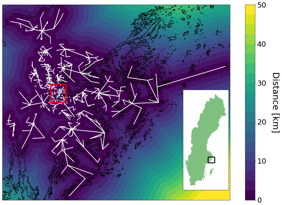
Figure 2Distribution of microwave links in Hi3G's Stockholm network. Here the white lines represent the links and the black lines the coast of Sweden around Stockholm. The colors in the legend represent the distance (km) per grid point to the closest link. The red square shows the selected sub-region at the city center. The inset shows the selected region within Sweden as a black square.
For Step 1, in this demonstration we assume that a user prefers maps with 250 m grid size and a time step (or accumulation period) of 1 min with acceptable ranges being 250–2000 km and 1–60 min, respectively. Furthermore, the user requests that the map quality is always QL ≥ 3 for 75 % of the land area. To evaluate this request, spatial resolutions of 250, 500, 1000 and 2000 m and accumulation times of 1, 2, 5, 15 and 60 min are tested. An example of distances to the closest link at 250 m resolution can be found in Fig. 2. The third step involves the characterization of the precipitation climate and here we illustrate the method using variograms for southern Sweden (van de Beek et al., 2020). The method described in this paper provides variogram shape as a function of day of the year and accumulation time, representing the average spatial correlation of precipitation in southern Sweden (for individual (extreme) rain events the shape of the variogram will generally differ).
Based on the precipitation climatology in this temperate climate region, in summer it is expected that the variograms have the shortest range due to convective precipitation. In winter, the range is expected to be longest with predominantly stratiform precipitation. An average situation can be expected in spring. We therefore evaluate the quality maps for three representative days of the year; 24 January (DOY 24), 15 April (DOY 115) and 25 July (DOY 206). In Fig. 1c the change in the range parameter of a spherical variogram throughout the year for different accumulation times is illustrated, using an example from the Netherlands. It should be noted that the variogram functions for Sweden, which are used in this demonstration of the methodology, were determined from 15 min up to daily resolution. Application of these functions for shorter accumulation times requires extrapolation. This might introduce inaccuracies, which are beyond the scope of this paper to quantify.
A selection of final quality maps for summer conditions (DOY 206) can be found in Fig. 3. Looking first at the highest-resolution map (250 m/1 min; Fig. 3a), the individual link locations are clearly visible as the representativeness of a link for its surrounding is very low at the 1 min scale. When moving to longer time steps this representativeness increases rapidly and at 60 min accumulations QL ≥ 3 for most of Stockholm. When increasing the grid size, the image remains similar, but coarser. However, the odds of a second link being within the range of a grid cell center increases and this can be manifested by the number of grid cells with QL = 4 increasing with decreasing spatial resolution.
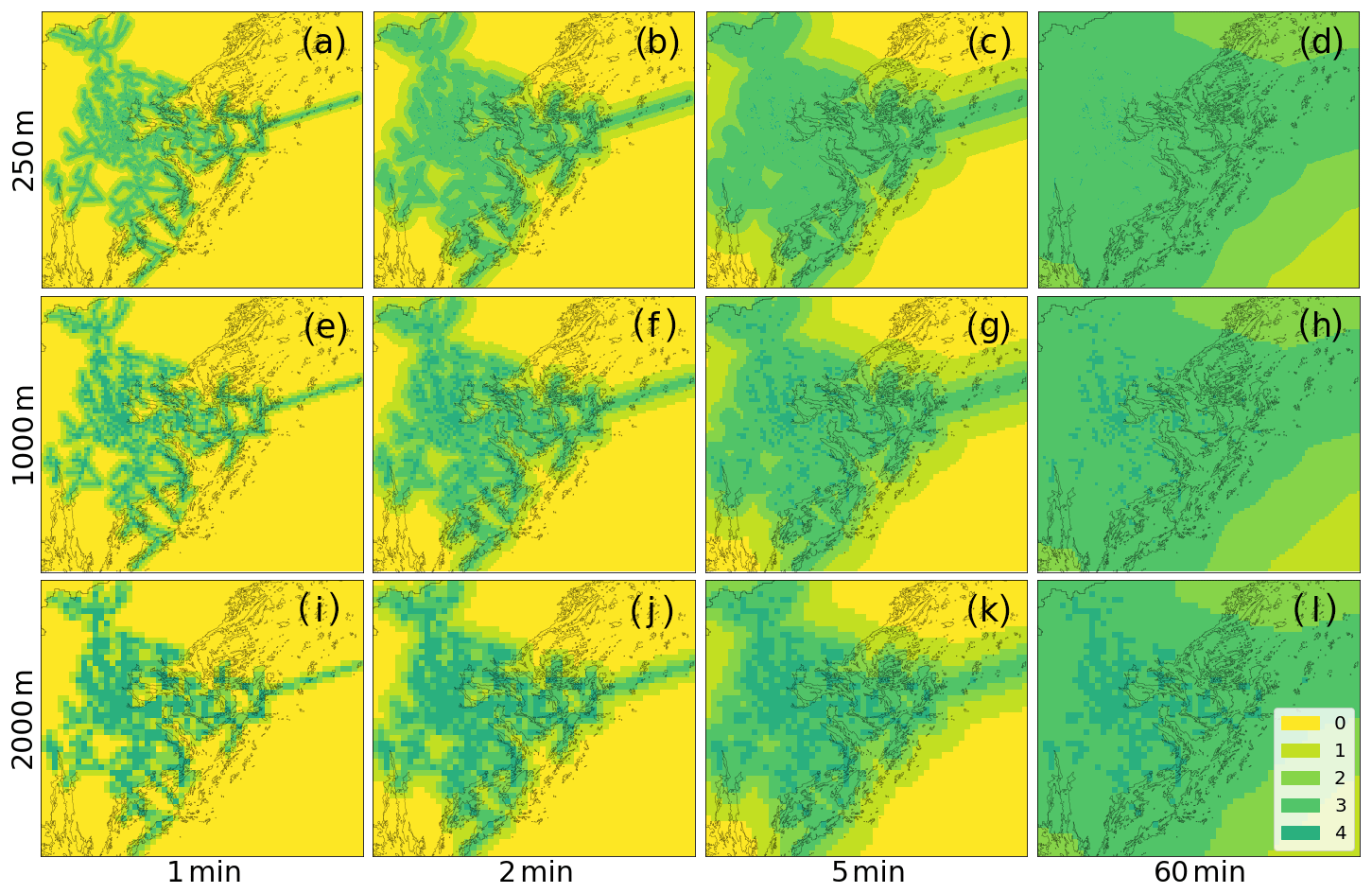
Figure 3Map of the attainable quality for different temporal and spatial resolutions using a variogram for southern Sweden in a summer situation (DOY 206), where the colors represent the quality levels equal to Fig. 1a and b. The columns represent the accumulation time (1, 2, 5, 60 min) and the rows the spatial resolution (250, 1000 and 2000 m). The map covers the entire Stockholm area, i.e. the full extent of Fig. 2.
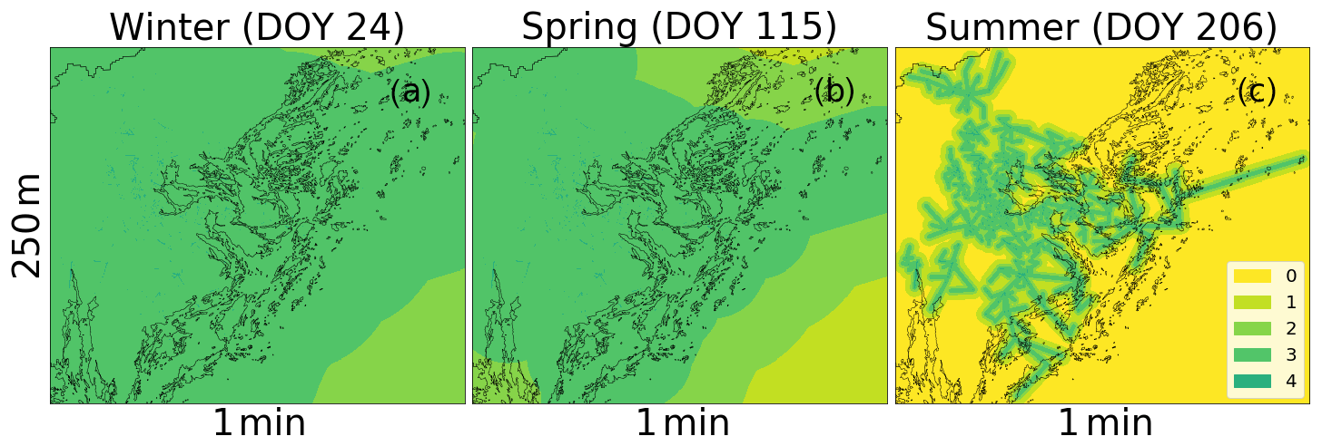
Figure 4Map of the attainable quality at 1 min and 250 m resolution for (a) winter (b) spring, and (c) summer precipitation regimes. The colors represent the quality levels equal to Fig. 1a and b.
How the attainable quality changes throughout the year is illustrated in Fig. 4, where winter, spring and summer situations are shown for an accumulation time of 1 min and spatial resolution 250 m. In winter, almost the entire domain is categorized as high quality (QL ≥ 3), reflecting the spatially correlated character of winter precipitation (Fig. 4a). In spring, the high-quality area decreases (Fig. 4b) and becomes very similar to the map obtained in summer for 250 m and 60 min resolutions (Fig. 3d), which well illustrates how the CML network, grid resolutions and precipitation processes interact to define the attainable quality. Finally, in the summer map the high-quality area is restricted to the vicinity of the links, reflecting the localized character of summer precipitation (Fig. 4c) As mentioned before, the time of the year is clearly very important for determining the potential quality of the map due to the different dominant processes.
Table 1Percent of grid cells (above land) within the study area (i.e. the full extent of Fig. 2), in three quality level categories (QL ≤ 1, QL = 2 and QL ≥ 3, summarized to improve readability of the table) at all temporal and spatial resolutions investigated, and for winter, spring and summer precipitation regimes.
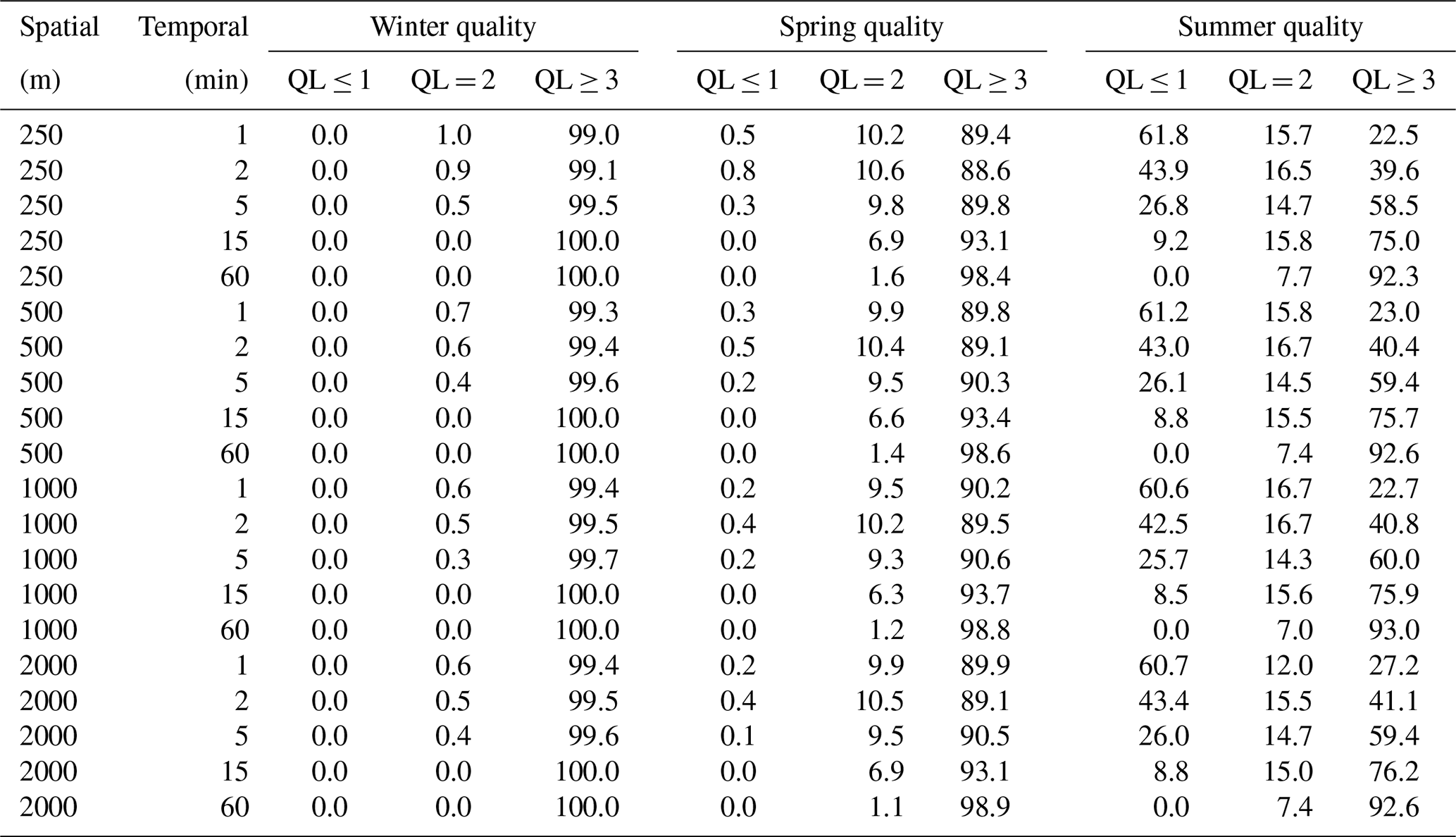
Table 1 shows a summary of the statistics of all grid cells that are over land for the three seasonal dates. Here the quality levels have been reduced to three to improve readability; QL ≤ 1 (low), QL = 2 (medium) and QL ≥ 3 (high). With the 75 % threshold, during winter a spatial resolution of 250 m and temporal resolution of 1 min is easily attainable as 99 % of the grid cells are marked as high quality. During spring these values become slightly lower, but still it is possible to have an acceptable map at this high resolution. However, for summer the results are quite different. At the 250 m resolution the 75 % threshold is only reached at time step 15 min. Even upscaling to a larger grid size has limited effect, which is partially because QL3 and 4 were grouped together. While a lot of grid cells were moved from QL3 to 4 only a limited number of grid cells were moved from QL2 to 3, resulting in very little visible changes in this table. In this example it therefore does not make much difference in changing the spatial scale, which is in agreement with the finding of de Vos et al. (2019), who concluded that resolution dependency is larger in time than in space. For the user to be on the safe side it could be recommended to choose map resolutions of at least 250 m and 15 min. Alternatively, the map resolutions can be changed depending on the time of the year. The choice of the extent of the map also has a large impact on the final results. When only looking at the city center (the red square in Fig. 2), the quality becomes much higher as the network density is greater. This is summarized in Table 2. Here it can be seen that even at the 250 m and 1 min resolution the 75 % threshold QL ≥ 3 is met in summer.
Table 2Percent of grid cells (above land) within the city centre (red square in Fig. 2), for each quality level category for a summer situation (DOY 206) at 250 and 1000 m and 1, 2, 5, 15, and 60 min resolutions.
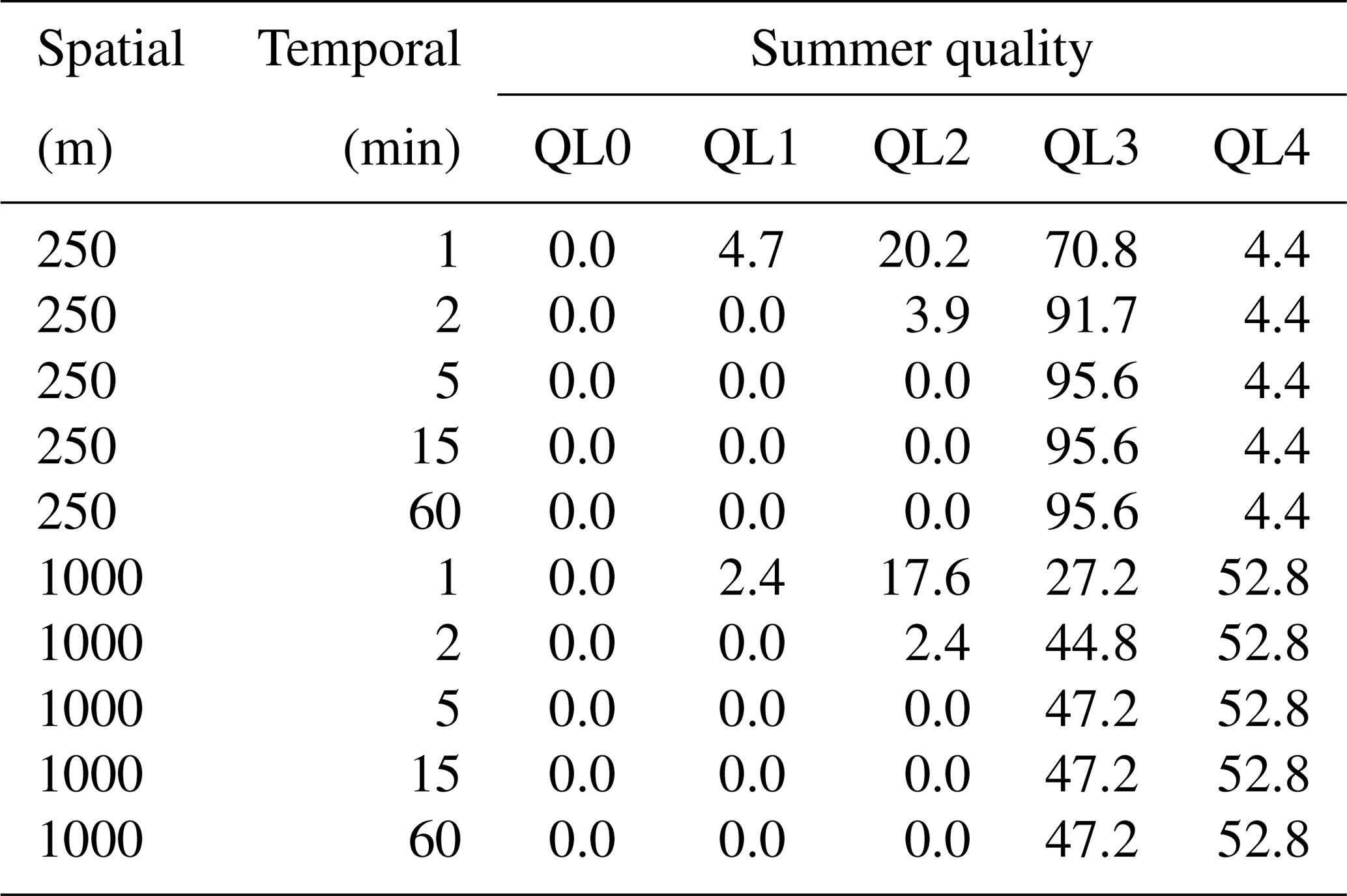
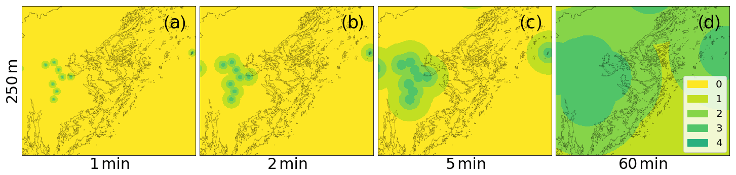
Figure 5Map of the attainable quality at 1, 2, 5, 60 min and 250 m resolution summer precipitation regime (DOY 206) using rain gauges and a variogram for southern Sweden. The colors represent the quality levels equal to Fig. 1a and b.
Finally, to illustrate that the same method can also be applied to point observations, Fig. 5 shows the results from an application of the method to the current operational gauge network in Stockholm. The results indicate that, during summer, the current rain gauge network density is not high enough to meet the 75% criterion up to hourly time scales. This illustrates the gain in quality that is potentially attainable by using CML networks for precipitation monitoring. The real gain in operational applications depends on a number of additional factors that require further research and development (see Sect. 4).
To conclude, we have demonstrated a method to identify the potential resolutions of precipitation estimates from CML networks. The method is simple, fast, transparent and conceivably useful e.g. for feasibility studies in regions considering CML-based precipitation observations. The method can be used to indicate the suitability of the data for different subsequent applications, requiring different resolutions (e.g. estimation of sewer overflows or treatment plant inflows in an urban hydrological context) in different seasons. Another potential application includes assessing the impact of malfunctioning links (i.e. operational network monitoring). We have demonstrated the method with a focus on a CML context, assuming line measurements, but it was shown to be equally applicable to point observations from, e.g., a precipitation gauge network.
A key limitation, when applying the method to CML-based observations, is that perfectly accurate measurements from the CML network are assumed, which is still not practically attainable, although much research is currently focusing on this topic. Such errors vary greatly in operational applications and can be significant (Andersson et al., 2017). If the measurement error of individual links is known it is possible to add this information as an additional dimension in the quality maps, which would address the uncertainty of category one (measurement errors) in Rios Gaona et al. (2015). This also applies to microwave link properties that are known to be error prone, e.g. short links or links crossing water. Moreover, another methodological limitation is that only two observations per grid cell are taken into account, although the number of observations and the distribution of the observations within a grid cell should have some influence. Additionally, the link length – particularly the spatial distribution of precipitation along the link paths – is not taken into consideration, which can lead to overestimation of quality level, especially for long links near the boundaries of the study area. One solution might be to take into account the end points of the line instead of the shortest distance to the link path. Another potential solution to this issue might be to use variogram information, as this could potentially be used to describe variability and uncertainty on individual link level, e.g. by applying directional variograms to reduce the impact of the Gaussian assumptions at shorter time-scales. Improving the method in these respects is clearly possible, although it makes the method much more complex to communicate to a user. Additionally it is not certain that the added value for the user will be significant.
The methodology was illustrated by using an example dataset. The exact locations of the microwave links and municipal rain gauges are currently not publicly accessible as they are part of a non-disclosure agreement. SMHI-operated gauge locations are available from the open data site of SMHI at: https://www.smhi.se/data/meteorologi/ladda-ner-meteorologiska-observationer#param=precipitation15MinutesSum,stations=active (last access: 15 June 2020) (SMHI, 2020).
RvdB and JA developed the methodology. The application of methodology and creation of figures were performed by RvdB. Most of the paper was written by RvdB with contributions of JO. Proofreading was performed by all three authors.
The authors declare that they have no conflict of interest.
This article is part of the special issue “19th EMS Annual Meeting: European Conference for Applied Meteorology and Climatology 2019”. It is a result of the EMS Annual Meeting: European Conference for Applied Meteorology and Climatology 2019, Lyngby, Denmark, 9–13 September 2019.
The authors would like to thank Vinnova and SMHI for supporting this research within the MEMO project (2017-03297), the FutureCityFlow project (2017-01046), and the project “Innovativa observationer”. We would also like to thank Ericsson and Hi3G Sweden for providing a sample of the CML network in Stockholm and two reviewers for providing constructive criticism on the original manuscript. Finally we would like to thank Riejanne Mook for optimizing the code.
This research has been supported by the VINNOVA (grant nos. 2017-03297 and 2017-01046).
This paper was edited by Tanja Winterrath and reviewed by Martin Fencl and one anonymous referee.
Andersson, J. C. M., Berg, P., Hansryd, J., Jacobsson, A., Olsson, J., and Wallin, J.: Microwave links improve operational rainfall monitoring in Gothenburg, Sweden, in: 15th International Conference on Environmental Science and Technology, 31 August–2 September 2017, Rhodes, Greece, 2017.
Chwala, C. and Kunstmann, H.: Commercial microwave link networks for rainfall observation: Assessment of the current status and future challenges, Wiley Interdiscip. Rev.: Water, 6, e1337, https://doi.org/10.1002/wat2.1337, 2019.
de Vos, L., Overeem, A., Leijnse, H. and Uijlenhoet, R.: Precipitation estimation accuracy of a nation-wide instantaneously sampling commercial microwave link network: error-dependency on known characteristics, J. Atmos. Ocean. Tech., 36, 1267–1283, 2019.
Fencl, M., Rieckermann, J., Sýkora, P., Stránský, D., and Bareš, V.: Commercial microwave links instead of precipitation gauges: fiction or reality?, Water Sci. Technol., 71, 31–37, https://doi.org/10.2166/wst.2014.466, 2015.
Goldshtein, O., Messer, H., and Zinevich, A.: Precipitation Rate Estimation Using Measurements From Commercial Telecommunications Links, IEEE T. Signal Proc., 57, 1616–1625, https://doi.org/10.1109/TSP.2009.2012554, 2009.
Gossett, M., Kunstmann, H., Zougmore, F., Cazenave, F., Leijnse, H., Uijlenhoet, R., Chwala, C., Keis, F., Doumounia, A., Boubacar, B., Kacou, M., Alpert, P., Messer, H., Rieckermann, J., and Hoedjes, J. C. B.: Improving Rainfall Measurement in Gauge Poor Regions Thanks to Mobile Telecommunication Networks, B. Am. Meteorol. Soc., 97, 49–51, https://doi.org/10.1175/BAMS-D-15-00164.1, 2016.
Graf, M., Chwala, C., Polz, J., and Kunstmann, H.: Rainfall estimation from a German-wide commercial microwave link network: Optimized processing and validation for one year of data, Hydrol. Earth Syst. Sci. Discuss., https://doi.org/10.5194/hess-2019-423, in review, 2019.
Haese, B., Hörning, S., Chwala, C., Bárdossy, A., Schalge, B., and Kunstmann, H.: Stochastic reconstruction and interpolation of precipitation fields using combined information of commercial microwave links and rain gauges, Water Resour. Res., 53, 10740–10756, 2017.
Journel, A. G. and Huijbregts, C. J.: Mining Geostatistics, Academic Press, London, New York, 1978.
Leijnse, H., Uijlenhoet, R., and Stricker, J. N. M.: Precipitation measurement using radio links from cellular communication networks, Water Resour. Res., 43, W03201, https://doi.org/10.1029/2006WR005631, 2007.
Messer, H., Zinevich, A., and Alpert, P.: Environmental monitoring by wireless communication networks, Science, 312, 713, 2006.
Olsson, J., Arheimer, B., Borris, M., Donnelly, C., Foster, K., Nikulin, G., Persson, M., Perttu, A.-M., Uvo, C. B., Viklander, M., and Yang, W.: Hydrological climate change impact assessment at small and large scales: key messages from recent progress in Sweden, Climate, 4, 39, https://doi.org/10.3390/cli4030039, 2016.
Overeem, A., Leijnse, H., and Uijlenhoet, R.: Two and a half years of country-wide rainfall maps using radio links from commercial cellular telecommunication networks, Water Resour. Res., 52, 8039–8065, https://doi.org/10.1002/2016WR019412, 2016.
Rios Gaona, M. F., Overeem, A., Leijnse, H., and Uijlenhoet, R.: Measurement and interpolation uncertainties in precipitation maps from cellular communication networks, Hydrol. Earth Syst. Sci., 19, 3571–3584, https://doi.org/10.5194/hess-19-3571-2015, 2015.
Scheidegger, A. and Rieckermann, J.: Bayesian assimilation of rainfall sensors with fundamentally different integration characteristics, available at: https://github.com/scheidan/CAIRS-Tutorial (last access: 3 June 2020), 2014.
SMHI: Ladda ner meteorologiska observationer, available at: https://www.smhi.se/data/meteorologi/ladda-ner-meteorologiska-observationer#param=precipitation15MinutesSum,stations=active, last access: 15 June 2020.
van de Beek, C. Z., Leijnse, H., Torfs, P. J. J. F., and Uijlenhoet, R.: Seasonal semivariance of Dutch precipitation at hourly to daily scales, Adv. Water Resour., 45, 76–85, https://doi.org/10.1016/j.advwatres.2012.03.023, 2012.
van de Beek, C. Z., Andersson, J. A. M., and Olsson, J.: Precipitation variability in Sweden: A variogram perspective at different time scales, in preparation, 2020.
Willems, P., Olsson, J., Arnbjerg-Nielsen, K., Beecham, S., Pathirana, A., Bülow Gregersen, I., Madsen, H., and Nguyen, V.-T.-V.: Impacts of Climate Change on Precipitation Extremes and Urban Drainage Systems, IWA Publishing, London, UK, 2012.
Zinevich, A., Alpert, P., and Messer, H.: Estimation of precipitation fields using commercial microwave communication networks of variable density, Adv. Water Resour., 31, 1470–1480, https://doi.org/10.1016/j.advwatres.2008.03.003, 2008.