Multi-sensor analysis of monthly gridded snow precipitation on alpine glaciers

Accurate and reliable solid precipitation estimates for high mountain regions are crucial for many research applications. Yet, measuring snowfall at high elevation remains a major challenge. In consequence, observational coverage is typically sparse, and the validation of spatially distributed precipitation products is complicated. This study presents a novel approach using reliable daily snow water equivalent (SWE) estimates by a cosmic ray sensor on two Swiss glacier sites to assess the performance of various gridded precipitation products. The ground observations are available during two and four winter seasons. The performance of three readily-available precipitation data products based on different data sources (gauge-based, remotely-sensed, and re-analysed) is assessed in terms of their accuracy compared to the ground reference. Furthermore, we include a data set, which corresponds to the remotely-sensed product with a local adjustment to independent SWE measurements. We find a large bias of all precipitation products at a monthly and seasonal resolution, which also shows a seasonal trend. Moreover, the performance of the precipitation products largely depends on in situ wind direction during snowfall events. The varying performance of the three precipitation products can be partly explained with their compilation background and underlying data basis.

1 Introduction

Observations of solid precipitation (snowfall) at high elevations are important for many fundamental and applied scientific questions in, for example, glaciology, hydrology and water resource management (e.g., Hock et al., 2017, 2019; Viviroli et al., 2020). However, reliable observations at a high spatio-temporal resolution are sparse in high mountain regions. Technical challenges in harsh high mountain conditions limit the number and quality of observations (e.g., Nitu et al., 2018; Buisán et al., 2020). Gridded precipitation products provide an important alternative to in situ observations as they cover large areas at a high spatio-temporal resolution. However, they are also prone to large uncertainties, which are often difficult to assess (e.g., Sun et al., 2018; Zandler et al., 2019). Therefore, their reliability for specific local applications needs thorough assessment prior to their use and case-specific bias corrections.

This study presents a novel approach using temporally continuous and reliable ground observations taken on two alpine glaciers in Switzerland. With daily snow water equivalent (SWE) observations by a cosmic ray sensor (CRS), which has previously been evaluated with promising results (Kodama et al., 1975; Howat et al., 2018; Gugerli et al., 2019), we assess the performance of readily-available, spatially and temporally highly resolved gridded precipitation products. In this study, we only use specific Swiss products because global gridded data products typically have much lower spatial and temporal resolution not serving the main purpose of this study.

The investigated precipitation products are based on (i) a dense gauge network (RhiresD), (ii) a ground-based weather radar network combined with the gauge network (CombiPrecip) and (iii) the analysis of the high resolution non-hydrostatic numerical weather prediction model COSMO-1. They are all operationally compiled by MeteoSwiss, readily available and have a high temporal (daily) and spatial (1×1 km) resolution. Each of these products has its advantages. RhiresD has an applied topography- precipitation gradient (Schwarb, 2000). CombiPrecip is directly measurement-based by the ground-based weather radar network and benefits from the observations of the gauge network. COSMO-1 analysis produces physically consistent fields of meteorological variables. In addition to these three data products, we add a further data set based on CombiPrecip that is adjusted to independent end-of-season in situ observations of SWE (Gugerli et al., 2020).

Gridded precipitation products are evaluated by their agreement of snowfall amounts compared to the in situ measured new SWE amounts at a seasonal and monthly resolution. Moreover, prevailing in situ meteorological conditions such as wind direction, wind speed and air temperature are used to characterize snowfall events, which are over- or underestimated by the precipitation products.

2 Study site and data

2.1 Study site

The two glacier sites of this study are located in different parts of the Swiss Alps (Fig. 1). Glacier de la Plaine Morte (7.1 km²) is situated on the mountain divide between the Northern (Bernese) Alps and the Rhone valley. With small elevation gradients (2470 to 2830 m a.s.l.) it is the largest plateau glacier of the European Alps (Huss et al., 2013). Findelengletscher (12.7 km²) is located in the Southern Swiss Alps at the border with Italy and covers elevation bands from 2561 to 3937 m a.s.l. (GLAMOS, 2018; Gugerli et al., 2020).

Figure 1 Shown are the location and outlines of Plaine Morte and Findelen glaciers (cf. Fischer et al., 2014), the locations of the CRSs, the weather radar network, and the precipitation gauge network, including stations above 2000 m a.s.l. Coordinates refer to the Swiss system (EPSG:21781, maps provided by Swisstopo).

2.2 Automatic weather stations and the cosmic ray sensors (CRS)

On Plaine Morte (46.38^∘ N, 7.50^∘ E, 2689 m a.s.l.) and Findelen (46.00^∘ N, 7.87^∘ E, 3116 m a.s.l.) an automatic weather station was installed in October 2016 and October 2018, respectively. These stations provide hourly measurements of air temperature, wind speed and direction, air pressure, relative humidity and snow depth. In addition, hourly estimates of SWE are obtained by a CRS. The CRS is a neutron detector that counts the number of fast neutrons per hour that penetrate the snowpack. These neutron counts need to be corrected for changes in air pressure and incoming cosmic ray flux. The moderated neutron counts are smoothed with a 6 h running mean before they are converted to SWE. The conversion follows a negative exponential relationship, i.e., the fewer neutrons are counted per hour, the higher the SWE estimates (Gugerli et al., 2019). With a daily resolution, the CRS has shown a good agreement with a one-to-one relationship and a standard deviation of ±10 % compared to 13 manually obtained field observations on Plaine Morte (Gugerli et al., 2019, 2020).

Some technical issues on Plaine Morte resulted in several data gaps of temperature, humidity, wind speed and snow depth, which were substituted with measurements from nearby highly correlated stations (Gugerli et al., 2019, 2020).

2.3 Gridded precipitation data (RhiresD)

The gridded precipitation data (RhiresD) is compiled using approximately 420 quality-controlled gauges of the Swiss Federal observation network. The gauge network consists of heated pluviometers with a rocking mechanism (1518 H3 and 15188 Lambrecht) and with a weighing mechanism (Pluvio1 and Pluvio2 by Ott). The pluviometers are not surrounded with a wind shield and measure with a 10 min frequency and a minimum amount of 0.1 mm (MeteoSwiss, 2015). The pluviometers are horizontally evenly distributed, but strongly biased towards lower elevations with only few gauges located above 2000 m a.s.l. (MeteoSwiss, 2019).

The gridded precipitation product RhiresD is a result of an interpolation based on a climatological mean and a regionally varying precipitation-topography (Schwarb, 2000). It has several sources of errors; (i) measurement errors of the gauges, (ii) their spatial representativeness, which may result in significant interpolation errors, and (iii) an effective grid resolution coarser than the given grid spacing (approximately 15–20 km, cf. MeteoSwiss, 2019). These deficits need to be kept in mind when comparing to point observations. RhiresD has a grid resolution of 1×1 km and a daily temporal resolution covering the time period between 06:00 and 06:00 UTC (+1 d).

2.4 Ground-based radar-gauge observations (CombiPrecip, CombiPrecip-adj)

Switzerland has an operational ground-based weather radar network consisting of five polarimetric C-band Doppler radars (Germann et al., 2015). Weather radars track the backscatter of hydrometeors within the atmosphere, which are then converted to rainfall amounts. The weather radars suffer from a wide range of uncertainties caused by beam shielding, beam broadening with distance, ground clutter, hardware instability, wet radome attenuation, etc (e.g., Joss et al., 1990; Joss and Lee, 1995; Germann and Joss, 2004). To mitigate these uncertainties, radar measurements are typically merged with precipitation gauge observations. The radar-gauge composite used in this study (CombiPrecip) is an operational implementation of merging gauges (cf. Sect. 2.3) and radar observations by co-kriging with external drift (see Sideris et al., 2014, for more information).

As shown in Gugerli et al. (2020), CombiPrecip has a large bias compared to end-of-season glaciological surveys. Hence, an adjustment factor depending on glacier-specific mean field bias and in situ air temperature was proposed (Eq. (4) in Gugerli et al., 2020). We include this data set, which is CombiPrecip adjusted by independent in situ measurements, in our analysis. For Plaine Morte (Findelen), CombiPrecip-adj (P_{CPC_AF}) is the hourly CombiPrecip multiplied by a factor of 2.6 (3.7) for solid precipitation (temperature below −2 ^∘C) and a factor of one for liquid precipitation (hourly air temperature above 2^∘). Mixed-phase precipitation (air temperatures between −2 and +2^∘) is adjusted with a linearly interpolated factor between one and 2.6 (3.7). The phase-parameterization by temperature follows the suggestion of Kochendorfer et al. (2017), and is coherent with Gugerli et al. (2020).

2.5 Numerical weather prediction model (COSMO-1)

The numerical weather prediction model COSMO has been developed by the consortium for small-scale modeling, a collaboration of national weather services of several countries (COSMO, 2020). MeteoSwiss runs the non-hydrostatic deterministic numerical weather prediction model COSMO-1 operationally since March 2016 (MeteoSwiss, 2016). The model is run at a grid resolution of 1.1 km with the domain centered over Switzerland. Boundary conditions are provided by ECMWF HRES (COSMO, 2018). For a detailed description of the dynamics and numerics of COSMO (version 5.00), the reader is referred to Doms and Baldauf (2013). In this study, we use precipitation estimates from the COSMO-1 analysis provided at an hourly resolution. COSMO-1 analysis is derived by assimilating the latest forecast fields with a radar-only precipitation product, radiosondes, wind profiler, surface pressure, and aircraft observations. The radar-only precipitation product is produced by the same ground-based radar network as used in CombiPrecip (cf. Sect. 2.4).

3 Methods

3.1 Pre-processing precipitation data and SWE observations

From each precipitation product, precipitation estimates of the grid cell closest to the two automatic weather stations is extracted over time (see Gugerli et al., 2020, for more information). RhiresD, CombiPrecip, CombiPrecip-adj and COSMO-1 have different temporal resolutions, with RhiresD (daily) having the coarsest. To make these data sets comparable, total daily sums of CombiPrecip (P_CPC,d), CombiPrecip-adj (P_{CPC_AF,d}) and COSMO-1 (P_COSMO,d) are calculated for the time period between 06:00 and 06:00 UTC (d+1) of day d.

The CRS provides continuous hourly observations of SWE. To increase the precision of the instrument and to reduce the noise, the hourly observations are averaged over 24 h centered around 06:00 UTC. The time of 06:00 UTC was chosen to be coherent with the RhiresD data set. Because the CRS provides continuous data on the snowpack, the time series needs to be broken down to obtain daily changes of SWE. Therefore, the difference between 06:00 UTC of d and 06:00 UTC (d+1) is considered the in situ measured snowfall of day d (ΔSWE_d, mm w.e.). Figure S1 in the Supplement illustrates the derivation of daily SWE amounts and daily total precipitation sums. Breaking down the cumulative time series of SWE into daily amounts, negative and positive daily changes may occur that are caused by snowfall, deposition, snow drift, sublimation and snowmelt.

In further processing (see Sect. 3.2.2), we apply a threshold corresponding to the precision of the CRS (σ_SWE) as presented in Gugerli et al. (2019). The precision estimate of the CRS allows distinguishing between signal and noise within the time series. Because this study focuses on mass gain by precipitation events only, the threshold is applied to limit all noise and to exclude all negative mass changes that are related to other processes than precipitation.

The precision is derived by error propagation. All constant parameters and continuous observations (incoming cosmic ray flux, air pressure and neutron counts) are assigned with an estimated uncertainty, which is propagated through the non-linear equations that correct the raw neutron counts and convert them to SWE. The dominating source of uncertainty arises from the statistical error of the neutron count itself. The statistical error follows a Poisson distribution, where lower neutron counts (higher SWE) result in a lower precision (Gugerli et al., 2019). Generally, the precision is expected to be higher on Findelen than on Plaine Morte because of the higher neutron count rate, which is a consequence of the elevation difference between the two sites. Not quantified here are the errors induced by the correction parameterizations and the conversion function.

The precision of the CRS allows excluding noise. However, true events can also be lost, especially in deep snowpacks. In addition, random false signals may not be excluded by the precision estimate. To best-possibly assure that we only include daily changes of SWE that are related to precipitation events, a double conditional bias is introduced in Sect. 3.2.2. With this double conditional bias, the CRS and the precipitation products need to agree on precipitation event-days.

3.2 Bias calculation between SWE and precipitation

3.2.1 Integrated bias

An integrated end-of-season bias is derived using cumulative precipitation and SWE observations at the end of the accumulation season, typically around 30 April. The integrated bias is motivated by the fact that reliable SWE observations in high mountain regions are often limited to a few measurements in time, sometimes one manual observation per season only. These observations are temporally limited because of the logistical and financial efforts needed to obtain them in high mountain regions. The temporal evolution of SWE is then inferred by using precipitation amounts from nearby stations at lower elevations or from precipitation data sets. Nonetheless, the end-of-season measurement of the snowpack is an integrated observation, i.e., apart from precipitation, it also includes effects of wind redistribution, sublimation, and potentially mass loss by early snowmelt. In consequence, several types of errors are introduced into such a time series. The comparison of an integrated end-of-season bias (F_int) with an event-based bias can thus provide insights into potentially introduced errors.

A seasonal end-of-season integrated bias is computed as

$$\begin{array}{}\text{(1)}& F_{\mathrm{int},\mathrm{w}}={\displaystyle \frac{P_{\mathrm{w}}}{{\mathrm{SWE}}_{\mathrm{w}}}}\end{array}$$

for each winter season with available observations. In our study, the end-of-season SWE (SWE_w) of winter w corresponds to the measurement obtained on 30 April by the CRS, while precipitation (P_w) is accumulated over the accumulation season. The beginning of the accumulation season is determined by the onset of the temporally continuous snowpack as observed by the CRS. Once the snowpack is established, we assume that further solid and liquid precipitation will build on the snowpack or refreeze within it, respectively. Snowmelt resulting in a net mass loss at these sites is assumed to be small until late April (Gugerli et al., 2019).

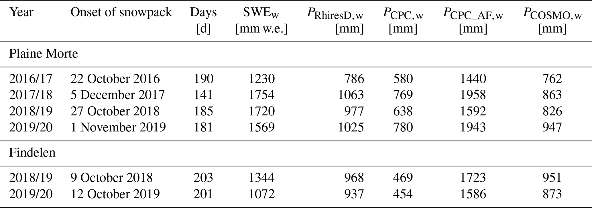
In consequence of the time period definition, each winter season is based on a different number of days (Table 1). By only considering the time period between the onset of the snowpack, i.e., from the moment the seasonal snowpack persists until 30 April, we limit the number of event-days that did not contribute to the snowpack because precipitation was liquid or because the accumulated snowfall melted again.

On Plaine Morte, no observations were available in October and November 2017. Hence, the onset of the snowpack could not be estimated and is defined as the date when measurements restarted. Another technical issue interrupted SWE observations on 26 April 2018, further shortening the 2017/18 winter season on Plaine Morte.

Table 1 Onset of the snowpack, number of days from the onset until 30 April (26 April for winter 2017/18 on Plaine Morte) and end-of-season amounts for the stations on Plaine Morte and Findelen. The end-of-season amounts are based on in situ SWE observations (SWE_w) and cumulative precipitation of RhiresD (P_RhiresD,w), CombiPrecip (P_CPC,w), CombiPrecip-adj (P_{CPC_AF,w}) and COSMO-1 (P_COSMO,w).

Additionally, we derive an overall integrated bias by dividing the sum of all end-of-season cumulative precipitation amounts by the sum of all SWE measurements obtained at the end of the season as

$$\begin{array}{}\text{(2)}& F_{\mathrm{int}}={\displaystyle \frac{\sum _{\mathrm{w}=\mathrm{1}}^n{P}_{\mathrm{w}}}{\sum _{\mathrm{w}=\mathrm{1}}^n{\mathrm{SWE}}_{\mathrm{w}}}}.\end{array}$$

To identify environmental conditions that result in a smaller or larger integrated end-of-season bias, daily air temperature (mean, minimum and maximum), wind speed (mean), wind gust (mean and maximum) and relative humidity (mean, minimum and maximum) are averaged over the same accumulation season (Table S1 in the Supplement). Seasonal averages of both glaciers and all winter seasons (six observations) are correlated with the end-of-season integrated bias of each winter season with a Pearson correlation and a significance level of 0.05. Moreover, these seasonal averages are also correlated with the relative difference between the integrated and conditional biases (Sect. 3.2.2).

3.2.2 (Double) conditional bias

A conditional bias is calculated for each winter seasons and month during the whole time period with available in situ observations on the two glacier sites. To analyse the seasonality of the bias, all months of all winter seasons are aggregated to derive the conditional seasonal monthly bias. Moreover, all snowfall event-days are categorized by wind direction measured on the glacier site. For each wind direction category, a bias is calculated.

The conditional bias (F_cond) is calculated by dividing the sum of daily precipitation totals by the sum of daily ΔSWE_d amounts as

$$\begin{array}{}\text{(3)}& F_{\mathrm{cond}}={\displaystyle \frac{\sum _{\mathrm{e}=\mathrm{1}}^n{P}_{\mathrm{e}}}{\sum _{\mathrm{e}=\mathrm{1}}^n\mathrm{\Delta }{\mathrm{SWE}}_{\mathrm{e}}}}\end{array}$$

where e is an event-day. This bias metric was previously employed in radar-derived precipitation studies (e.g., Germann et al., 2006; Speirs et al., 2017; Gabella et al., 2017). We refer to this bias as “(double) conditional” because an event-day fulfills two threshold criteria, one on ΔSWE_d and one on P_d. Event-days are therefore assumed to only include precipitation events and exclude all SWE increases that may be caused by other accumulation processes or by the noise of the CRS.

The threshold applied to daily SWE amounts (ΔSWE_d) is determined by its precision (σ_SWE,d, see Sect. 3.1). Since σ_SWE,d has values between 0.6 and 16.4 mm, daily precipitation estimates need a threshold, too. For daily precipitation totals, a threshold of 0.3 mm d⁻¹ is applied. This threshold has been applied in previous studies investigating radar-derived precipitation products (e.g., Germann et al., 2006).

An event-day is defined with ΔSWE_d greater than σ_SWE,d and P_d greater than 0.3 mm d⁻¹. The precipitation threshold is mostly lower than σ_SWE,d resulting in two important setbacks. First, the number of event-days is mainly dictated by the CRS observations. Second, the difference in thresholds allows for a potentially higher underestimation of precipitation. The sensitivity of the results with respect to the thresholds is further analysed by performing all calculations with three additional thresholds that are equal for precipitation and SWE. These thresholds are 0.0 mm d⁻¹, 0.3 mm d⁻¹ and σ_SWE,d.

The event-days are always defined in the same way for all conditional bias, independent of temporal resolution. Nonetheless, they vary among the precipitation data sets. The difference between the conditional biases lies within the aggregation of these event-days, which is either by the accumulation season, the individual months, the month of the year (aggregated) or the wind direction.

For the end-of-season conditional bias, event-days within the accumulation season, i.e., from onset of the snowpack to 30 April of each season (Table 1), are included to be coherent with the integrated end-of-season bias.

In the monthly conditional bias, the number of contributing event-days varies with month, season and glacier. On Plaine Morte (Findelen), 25 (14) months with measurements are available. To render the correlations of the monthly bias with daily air temperature, air humidity and wind speeds more robust, only months with more than two event-days are considered. This excludes December 2016 and April 2018 on Plaine Morte and January 2020 on Findelen. The conditional seasonal monthly bias is derived by aggregating all event-days by the month of the season. For example, the seasonal monthly bias of December is derived by all event-days from December 2016–2019 on Plaine Morte. It is a more robust estimate of the bias compared to averaging the monthly bias over all years.

In addition, we analyse the influence of wind direction by categorizing wind direction into four main sectors; North, East, South and West. Each wind sector has a size of 90^∘ centered around the main wind direction. For example, wind sector “South” includes all event-days with wind directions between 135^∘ (southeast) and 225^∘ (southwest). The daily wind directions of event-days are derived by averaging the meridional and zonal components of wind speed and -direction during all reported precipitation hours of CombiPrecip, CombiPrecip-adj and COSMO-1. For RhiresD, only daily amounts are availabe and therefore, wind direction is averaged over the entire day. The conditional bias is calculated with Eq. (3) with the difference that event-days are not aggregated by a time system, but by the wind sector category. The data gap from end of January 2018 to beginning of April 2018 for wind direction on Plaine Morte results in the loss of up to 22 event-days as identified by COSMO-1.

The uncertainty of all conditional biases are estimated by a leave-one-out cross validation with the mean absolute difference to the reference value. This uncertainty estimate, however, does not include a constant bias of the CRS nor the error arising from comparing a point estimate to a grid cell estimate.

4 Results and discussion

4.1 Integrated vs. (double) conditional end-of-season bias

The end-of-season precipitation biases vary over the different winter seasons, the two glacier sites and the analysed precipitation products (Fig. 2). Precipitation during the winter season 2016/17 on Plaine Morte, which has the lowest SWE over all winter seasons, is, for example, less underestimated than in other winter seasons. For RhiresD and COSMO-1, precipitation in the winter season 2018/19 is more underestimated than in other seasons, but does not show the highest end-of-season SWE (Table 1). Nonetheless, these two precipitation products show a significant correlation (RhiresD; r²=0.67, COSMO-1; r²=0.82) between the integrated bias and the end-of-season SWE amounts based on the six observations from Findelen and Plaine Morte. Further significant correlations between the integrated seasonal bias and the seasonal meteorological parameters were found for daily maximum temperature (CombiPrecip, r²=0.66) and daily relative air humidity (COSMO-1, r²=0.71). CombiPrecip performs slightly better with higher air temperatures that are still below 0 ^∘C. Especially the winter seasons of 2016/17 and 2019/20 on Plaine Morte were warmer than the other seasons. Finally, the integrated bias is closer to a factor of one for COSMO-1 with lower relative humidity. In contrast, the integrated bias of COSMO-1 shows no significant correlation with the number of precipitation days reported by COSMO-1 (single conditional). Hence, the integrated bias of COSMO-1 is smaller when the winter is characterized by lower relative humidity and not necessarily with fewer precipitation event-days. This indicates that in a drier season where sublimation rates may be stronger, the integrated bias is lower and underestimation consequently weaker.

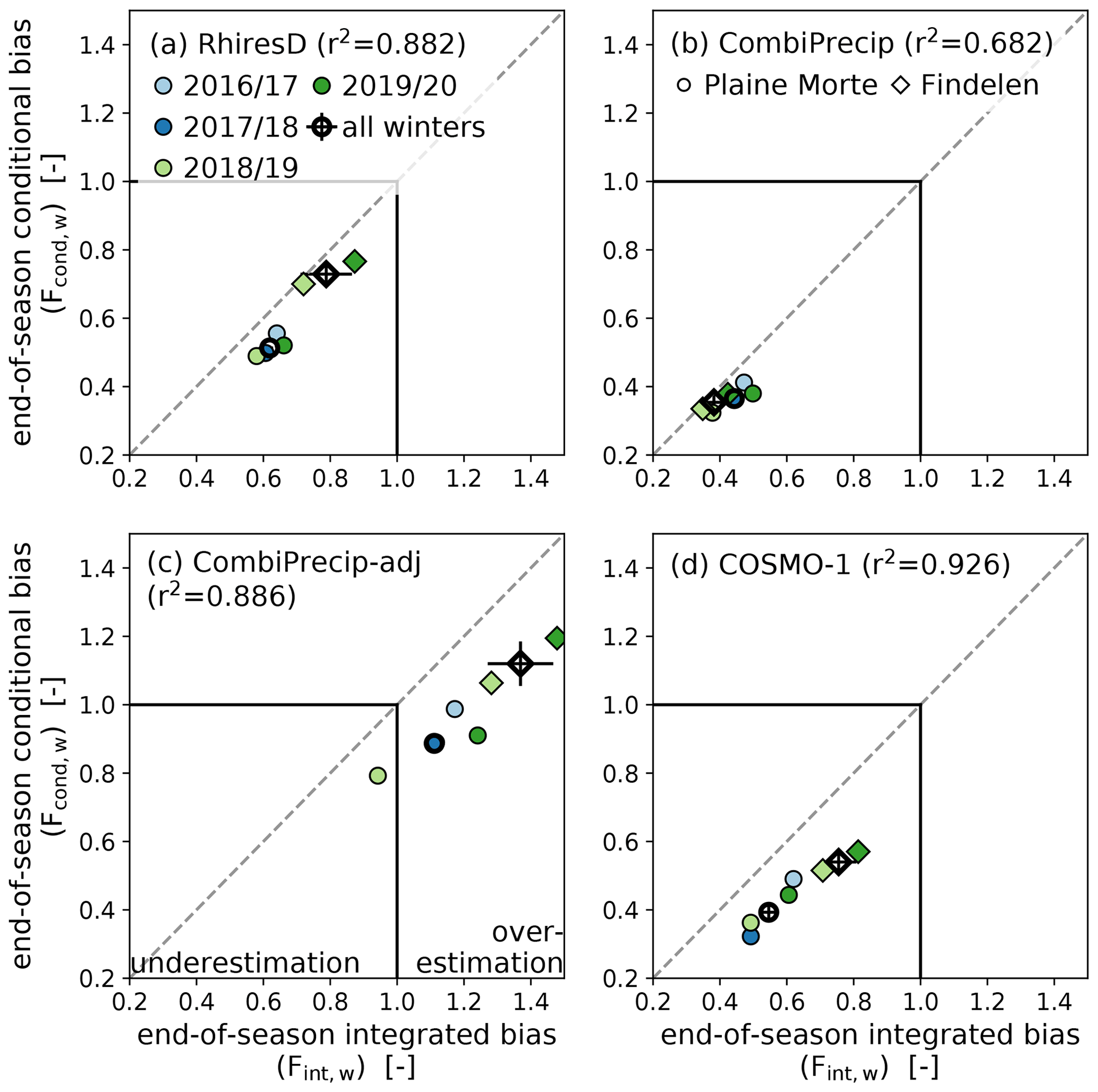
Figure 2 End-of-season bias derived with the accumulated (integrated) SWE amounts and cumulative precipitation during the accumulation season (F_int,w), and derived based on event-days during the accumulation season (conditional bias, F_cond,w) for the precipitation products (a) RhiresD, (b) CombiPrecip, (c) CombiPrecip-adj and (d) COSMO-1. On Plaine Morte, four winter seasons (2016/17–2019/20), and on Findelen two winter seasons (2018/19–2019/20) are available. The dashed grey line shows a one-to-one correlation. Values below (above) one show an underestimation (overestimation) of precipitation compared to in situ SWE observations (black solid lines). The uncertainty of the bias over all winter seasons (F_int, F_cond) is calculated with a leave-one-out cross validation.

The integrated and conditional biases are highly correlated for P_COSMO (r²=0.926) and moderately correlated for P_CPC (r²=0.68, Fig. 2). The overall end-of-season integrated bias (F_int), which contains processes such as snow drift, sublimation and potentially early snowmelt, has values between 0.44 (P_CPC) and 1.11 (P_{CPC_AF}) on Plaine Morte and between 0.38 (P_CPC) and 1.37 (P_{CPC_AF}) on Findelen. If we derive a bias based on precipitation event-days only (conditional bias, F_cond), the bias becomes larger and underestimation becomes more pronounced for almost all data sets; On Plaine Morte, the range is from 0.36 (P_CPC) to 0.89 (P_{CPC_AF}) and on Findelen from 0.35 (P_CPC) to 1.12 (P_{CPC_AF}). The adjustment with independent in situ observations to CombiPrecip (CombiPrecip-adj, P_{CPC_AF}) results in an average overestimation of the in situ SWE on Findelen (30 %–50 %) for all winter seasons and on Plaine Morte (10 %–30 %) for most winter seasons (Fig. 2c).

The relative difference between the integrated and conditional bias is significantly correlated with air humidity for P_RhiresD (r²=0.67). A low seasonal relative humidity of around 65% (winter 2018/19 on Findelen, Table S1) results in a small difference of 3 % between the integrated and conditional bias while the difference is approximately 20 % for a seasonal relative humidity of more than 80 % (winter 2017/18 and 2019/20 on Plaine Morte). With higher air humidity, the integrated bias underestimates less than the conditional bias. Another significant correlation (r²=0.80) is found for P_COSMO with daily wind gusts averaged over the accumulation season. Winter 2017/18 on Plaine Morte is characterized with seasonal average wind gusts of 9.2 m s⁻¹ (Table S1). In the same season, the integrated bias has a value of 0.49 and the conditional bias has a value of 0.32, which corresponds to a difference of 34 %. In contrast, winter 2016/17 on Plaine Morte shows average wind gusts of 6.9 m s² and a relative difference of 21 %. The integrated and conditional bias of the other winter seasons on Plaine Morte and Findelen differ less than 30 %, while the seasonal average of daily mean wind gusts are between 7.2 and 7.6 m s⁻¹.

The difference between the integrated and conditional overall end-of-season bias is sensitive to the threshold applied. In the following, we refer to the reference threshold as the one in the main analysis (P_d>0.3 mm d⁻¹ and $\mathrm{\Delta }{\mathrm{SWE}}_{\mathrm{d}}>{\mathit{\sigma }}_{\mathrm{SWE},\mathrm{d}}$). Applying a threshold of 0.0 or 0.3 mm d⁻¹ to the daily precipitation and SWE results in conditional biases that are between 11 % (P_RhiresD) and 27 % (P_COSMO) larger than the integrated bias for Plaine Morte (Fig. S10), indicating more underestimation. On Findelen, the threshold of 0.3 mm d⁻¹ results in biases that differ less than 3% from the integrated bias for P_RhiresD and P_CPC. For P_{CPC_AF} and P_COSMO this conditional bias differs 15 % and 25 % from the integrated bias, respectively. In all cases, the conditional bias indicates more underestimation than the integrated bias with these thresholds.

With a high threshold of σ_SWE,d applied on precipitation as well as SWE, the resulting conditional bias is 7 % (P_RhiresD) and 12 % (P_CPC) smaller than the integrated bias on Plaine Morte, indicating less underestimation. For the other precipitation products, it differs less than 4 % from the integrated bias. On Findelen, an end-of-season conditional bias of one is obtained for P_RhiresD with the common threshold of σ_SWE,d. The event-days included in this conditional bias have precipitation amounts greater 1.3 mm d⁻¹ with an average of 28.6±28.8 mm d⁻¹. In general, event-days with daily precipitation amounts greater than 0.6 mm d⁻¹, which corresponds to the lowest σ_SWE,d of the double conditional event-day, have a better agreement with in situ observations for all precipitation products. However, the number of events and the total precipitation as well as SWE amounts are strongly reduced with this high threshold. The excluded light precipitation events contribute more than 20 % to the end-of-season total precipitation amounts. In addition, up to 80 % of the event-days as identified by the individual precipitation products (single conditional) are excluded (Fig. S10c and d).

In conclusion, if only one observation in time is available and the goal is to infer snow accumulation at a higher temporal resolution, adjusting precipitation amounts with the integrated end-of-season bias may be justified and has shown good results (e.g., Huss and Fischer, 2016; Gugerli et al., 2019, 2020). Only considering precipitation event-days is sensitive to the thresholds applied and shows that by only including strong precipitation events, the conditional bias and the integrated bias are similar. Considering all precipitation event-days, in contrast, results in a stronger underestimation by the end-of-season conditional bias compared to the end-of-season integrated bias.

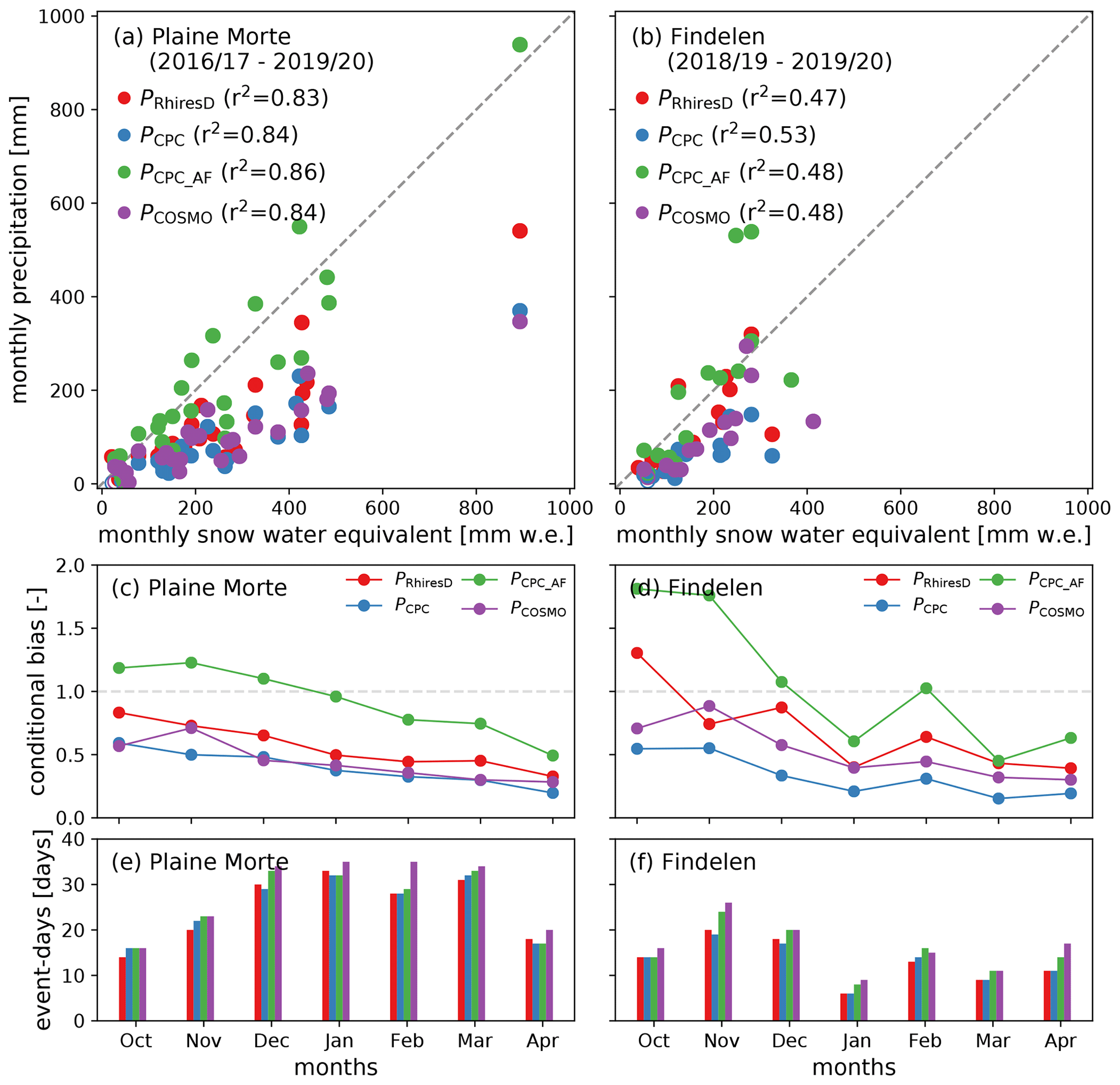
Figure 3 Panels (a) and (b) show the monthly precipitation and SWE totals on Plaine Morte and Findelen, respectively. Panels (c) and (d) show the conditional bias grouped for the month over four and two winter season on Plaine Morte and Findelen, respectively. The four (two) year sum of event-days of the given month are presented in (e) and (f) for Plaine Morte and Findelen, respectively. In (c) and (d) values below (above) one show an underestimation (overestimation) of precipitation amounts with respect to SWE.

4.2 The monthly (double conditional) bias and its seasonality

At monthly resolution, precipitation data sets and in situ SWE observations on Plaine Morte agree fairly well with r² values between 0.83 (P_RhiresD) and 0.86 (P_{CPC_AF}, Fig. 3a). Monthly totals lie between 20 mm w.e. (October 2016) and 890 mm w.e. (January 2018). On Findelen, generally lower monthly in situ totals are reported with a maximum of 400 mm w.e. (April 2019). The correlation is also lower with r² between 0.47 (P_RhiresD) and 0.53 (P_CPC, Fig. 3d). A double conditional bias on precipitation tends to worsen a correlation because of the removal of 0.0 mm d⁻¹ precipitation.

In general, the performance on Plaine Morte is better than on Findelen, partly due to the following reasons. A weather radar is located next to Plaine Morte and it is surrounded by several precipitation gauges in all four cardinal points. On Findelen, in contrast, precipitation gauges are only located in the west of the glacier. In addition, the quality of weather radar estimates is lower due to the following reasons. The larger distance between radar and target site results in more residual ground clutter and a poorer resolution caused by beam broadening. Most echoes on Findelen are rejected because they are considered to be ground clutter contaminated (Gugerli et al., 2020; Gabella and Notarpietro, 2002). In all radar applications, the term ground clutter refers to unwanted echoes from the ground. Although ground clutter cannot be completely eliminated, its effect can be mitigated with a careful design.

All precipitation data sets have a common trend throughout the accumulation season on both glaciers (Fig. 3c and d); a monotonically increase of the underestimation by precipitation during the accumulation season. CombiPrecip (P_CPC) has the highest bias on both glacier sites throughout the course of the winter season. Evidently, P_{CPC_AF} has a bias closest to a factor of one because it was adjusted with an unconditional bias (cf. Sect. 2.4). It also overestimates monthly in situ SWE amounts in the beginning of the season on both sites (Fig. 3c and d).

On Plaine Morte, more event-days are recorded from December to March than in October, November and April (Fig. 3e). For October and November, the measurement gap of winter 2017/18 most likely contributes to this fact. On Findelen, in turn, most event-days are reported in November (Fig. 3f) with only few event-days in January. Comparing the different precipitation data sets, it becomes clear that P_COSMO includes more event-days than the other data sets (Fig. 3e and f), while monthly sums remain similar (Fig. 3a and b).

An important aspect to note is the correlation of the precision of the CRS with the depth of the snowpack (Sect. 3.1). The deeper the snowpack, the less accurate the CRS becomes. Consequently, light snowfall event-days cannot be detected with a CRS, especially towards the end of the season with deep snowpacks. Accordingly, the lower threshold on the precipitation data sets may induce a stronger underestimation by the precipitation data set. To analyse this influence, the monthly biases were also calculated with thresholds of 0.0 mm d⁻¹ (Fig. S11), 0.3 mm d⁻¹ (Fig. S12) and σ_SWE,d (Fig. S13) applied on precipitation and SWE. For Plaine Morte, the results remain similar when a threshold of 0.0 mm d⁻¹ is applied on precipitation estimates as well as SWE. With the common threshold of σ_SWE,d, however, the linear trend over the winter season becomes weaker for Plaine Morte. This is especially pronounced for P_COSMO and P_CPC. Simultaneously, many event-days are removed, especially from January to April. On Findelen, only few events remain, and the statistics become less robust (Fig. S13).

4.3 The influence of wind direction

Figure 4 shows that wind direction has an important influence on whether a snowfall event is over- or underestimated by the precipitation data sets. For Plaine Morte, for example, P_RhiresD generally shows a stronger underestimation of SWE on event-days with winds from the north. The precipitation gauges located in the north of Plaine Morte are further away than the ones in the east, west and south. Because Plaine Morte is located on the weather divide between the Bernese Alps and the generally drier Rhone valley (see e.g., Fig. 6 in Isotta et al., 2014), gauges located further away are more likely to be located in another regional climate. This effect is not as pronounced in P_CPC and P_{CPC_AF} even though both data sets include the same gauge network. Hence, the radar observations compensate for the spatially non-continuous distribution of gauges.

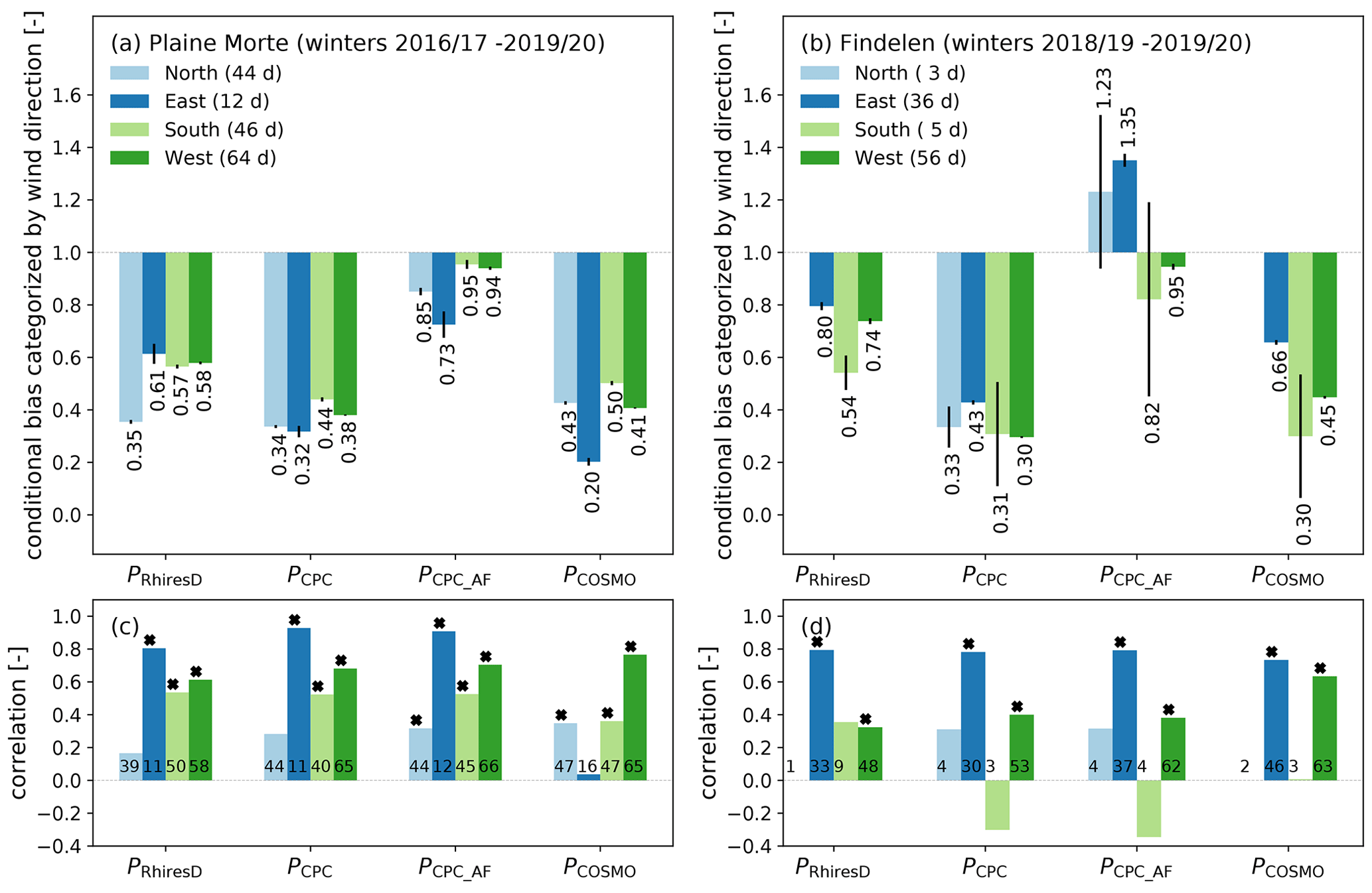
Figure 4 Conditional bias based on event-days and derived for the four main wind sectors on (a) Plaine Morte and (b) Findelen. The uncertainty is calculated with a leave-one-out cross validation. Numbers below the bars display the bias value in (a) and (b). Panels (c) and (d) show the correlation between precipitation and SWE estimates during the event-days within the wind sectors for Plaine Morte and Findelen, respectively. Significant correlations (α<0.05) are marked with a star. Numbers at the bottom of the bars correspond to the number of event-days per category and precipitation data set. The evaluation is only shown if more than two event-days are included.

Re-analysed precipitation (COSMO-1) has most inaccurate precipitation estimates with easterly winds on Plaine Morte (Fig. 4a and c). Two large event-days with easterly winds (29 October 2019 and 8 January 2018) increased SWE by more than 50 mm w.e. These events were better captured by P_RhiresD, P_CPC and P_{CPC_AF}. The re-analysed precipitation data (P_COSMO) reports less than 10 mm of precipitation for each of these events. On 27 October 2018, in contrary, in situ SWE increases by 2.8 mm w.e. while P_COSMO and P_RhiresD show amounts larger 20.0 mm. P_CPC and P_{CPC_AF} report no precipitation.

On Findelen, the performance of each precipitation data set is also related to the wind sectors (Fig. 4b and d). In contrast to Plaine Morte, precipitation event-days are mainly recorded for two wind sectors (east and west). More than half of the precipitation event-days are associated with winds from the west, and almost 40 % with winds from the east. On average, only very few event-days are associated with winds from the south and the north. Precipitation and SWE do not correlate significantly for events-days with southerly or northerly winds. In addition, the uncertainty is signficantly higher than for the other wind sectors.

It is also interesting to note that P_{CPC_AF} shows an overestimation for event-days with winds from east on Findelen (Fig. 4b). This is mainly dominated by a single precipitation event. The event on 29 Oct 2018 contributes 20 % to the total amount of P_{CPC_AF} within the eastern wind sector. During this event, P_{CPC_AF} reports 324 mm, which is almost three times as much as measured on the ground (120 mm w.e.) and implies a strong over-adjustment of P_CPC (cf. Sect. 2.4). The other data sets report 162 mm (P_RhiresD) and 125 mm (P_COSMO). Average wind speeds of that day are 9.6 m s⁻². However, not all event-days with high wind speeds result in an overestimation.

The bias aggregated by wind direction shows some sensitivity to the applied threshold (see Sect. 3.2.2). While the main wind directions during precipitation events are conserved and the main results, i.e., under which wind directions the performance of the precipitation products is better or worse shows little sensitivity, the calculated biases are more sensitive. On Plaine Morte, the biases are on average reduced by 10±13 % and 34±20 % for a common threshold on SWE and precipitation of 0.3 mm d⁻¹ and σ_SWE,d, respectively. For a threshold of 0.0 mm d⁻¹, the biases remain within a standard deviation of ±9 %. On Findelen, the biases are reduced by 9±11 % and 18±86 % for a threshold of 0.3 mm d⁻¹ and σ_SWE,d, respectively. For a threshold of 0.0 mm d⁻¹, the biases increase on average by 5±13 %. Furthermore, the performance of P_RhiresD improves substantially with a threshold of σ_SWE,d from an underestimation larger 20% with the reference threshold to an agreement within ±5 % with in situ SWE on Findelen. In addition, with a threshold of σ_SWE,d, the wind directions are reduced to east and west on Findelen only (Fig. S18). On Plaine Morte, the same threshold reduces the number of event-days with easterly winds but does not result in such a substantial difference of the performance of the precipitation products.

Correlating the bias based on monthly estimates (Fig. 3a and b) with average daily air temperature, air humidity and wind speed during event-days, the significant correlations are not the same for the different precipitation data sets or glacier sites. On Plaine Morte, all precipitation products show a significant correlation between air temperature and the monthly conditional bias based on 24 months, while only the biases of P_RhiresD and P_CPC are significantly correlated with humidity (r²=0.29 and r²=0.37, Fig. S14). The correlation with air temperature shows that a lower air temperature during snowfall has a larger bias. This negative correlation may be explained as follows; Above a certain threshold of air temperature on the glacier site, precipitation is assumed to be liquid at the gauge-sites included in RhiresD and ComibPrecip because they are located at lower elevations. In consequence, the gauge observations are more reliable because undercatch mainly affects solid precipitation (e.g., Nitu et al., 2018). COSMO-1 seems also to be able to model precipitation with higher temperatures more accurately. No significant correlation was found for wind speeds on Plaine Morte. On Findelen, the 13 months of available in situ measurements that also have more than two event-days show only a significant correlation with air temperature for P_RhiresD (r²=0.31, Fig. S15).

Generally, the dependence of the performance on synoptic situations indicated by in situ wind direction during snowfall events is in line with Lundquist et al. (2015). In addition, our results also show prevailing meteorological conditions, in which precipitation data sets overestimate in situ SWE amounts. Given the complex topography of the Swiss Alps and the distance between the two glacier sites, however, wind conditions on each glacier may strongly differ. Hence, it is not surprising that COSMO-1 struggles with winds from east on Plaine Morte, but performs best on Findelen with the same wind category.

4.4 General performance and limitations

A recent study by Lundquist et al. (2019) discusses the increasing improvements of numerical weather prediction models compared to interpolated gauge-observations. In our study, COSMO-1 performs better than RhiresD, which is gauge-based, in terms of bias and correlation on both glacier sites on a monthly resolution (Fig. 3). Nonetheless, COSMO-1 performs slightly worse compared to the measurement-based CombiPrecip and CombiPrecip-adj. The main advantage of CombiPrecip is shown with the different wind directions. While the bias of RhiresD and COSMO-1 is sensitive to wind direction, CombiPrecip is not, especially not on Plaine Morte. The gauge-based precipitation data set (RhiresD) generally performs well, but its performance depends on the gauge location with respect to the target site, the altitude and the precipitation phase at the gauge site.

Given the challenging environmental conditions for direct observations of SWE and/or snowfall on the two glacier sites of this study, the CRS provides the highest possible data quality and reliability. Limitations of the CRS observations are given by the noise, which depends on the depth of the snowpack, and the continuous cumulative time series, which needs to be transformed to an instantaneous measurement coherent with the precipitation estimates. This transformation is not straightforward because of the noise included in the observations. To increase confidence within the daily continuous estimates before the daily changes are calculated, we derive a daily average centered around 06:00 UTC (Sect. 3.1). This average comes with a time lag with regard to precipitation, i.e., it also includes potential snowfall of the previous and subsequent days (Fig. S1). However, a daily average centered around 12:00 or 18:00 UTC generally decreases the correlation between daily SWE and precipitation sums (not shown).

An aspect that needs to be addressed is the sensitivity of these results to the thresholds used to calculate the double conditional bias. The threshold applied for the main result (P_d>0.3 mm d⁻¹ and $\mathrm{\Delta }{\mathrm{SWE}}_{\mathrm{d}}>{\mathit{\sigma }}_{\mathrm{SWE},\mathrm{d}}$) is different for SWE and precipitation. This difference allows for a potentially stronger underestimation by the precipitation products because the threshold is generally lower for precipitation than for daily SWE. Evidently, this would not matter if precipitation and SWE would perfectly agree. But as other studies with the same or similar precipitation data products show, an underestimation is to be expected on glacierized high mountain sites (e.g., Huss and Fischer, 2016; Gugerli et al., 2019, 2020). A sensitivity analysis of the main results by including three additional thresholds that are equal for precipitation and SWE (0.0 mm d⁻¹, 0.3 mm d⁻¹ and σ_SWE,d) show that the underestimation is generally reduced (Sect. 4.1–4.3) with a high threshold (σ_SWE,d). Higher thresholds affect the total amounts of end-of-season SWE more than the total precipitation amounts at the end of the season (Figs. S2–S10). Consequently, in situ SWE is less underestimated by the precipitation products on Plaine Morte with a higher threshold. However, it also limits the analysis to event-days with stronger precipitation totals and light precipitation events are not considered. While a higher threshold results in an improvement for almost all precipitation products on Plaine Morte and Findelen, this does not apply for CombiPrecip-adj on Findelen (Fig. S8d). Estimates of CombiPrecip-adj increase with a higher threshold resulting in a stronger overestimation of SWE. Besides the bias between SWE and precipitation, the correlation between daily SWE and precipitation decreases with a higher threshold (Figs. S2–S10). For example, the correlation between SWE and precipitation by RhiresD results in an overall correlation of 0.60 (258 event-days) and 0.56 (154 event-days) with an equal threshold of 0.0 and 3.0 mm d⁻¹, respectively (Fig. S2a and b). This sensitivity is similar for all precipitation products (Figs. S2–S10).

Another important limitation is the spatial representativeness of these results. Only two sites with point observations are available for this study and they significantly differ with respect to topography and the regional climatic conditions. Furthermore, we compare point estimates to a grid cell of at least 1×1 km. Therefore, care needs to be taken with this approach as the in situ estimate may not be representative for a grid cell (e.g., Fassnacht et al., 2018). On Plaine Morte, the spatial variability of snow depth and snow density over the glacier is, however, small (Huss et al., 2013) and therefore, the station is considered representative for a grid cell and the glacier-catchment. On Findelen, in turn, spatial variability of snow accumulation is large, but repeated end-of-season spatial patterns of three subsequent years reveal a consistent spatial pattern of snow accumulation (Sold et al., 2016).

Moreover, the assessment of the bias between in situ SWE observations and precipitation will most likely not apply to non-glacierzied mountain sites, in particular to wind-blown crests. Glaciers typically form in places that are either snow-rich or cold throughout the year, and snow accumulation lasts several summer seasons. In addition, CombiPrecip-adj only exists for selected glacier sites (cf. Gugerli et al., 2020), therefore, it is strongly limited in space. Despite these limitations, the results reveal important aspects of the investigated precipitation data sets.

5 Conclusions and perspectives

A wide range of studies focus on improving precipitation estimates in high mountain regions using various approaches, in situ observations and/or geostatistical interpolation methods. However, validating solid precipitation estimates in high mountain regions remains a challenge and typically includes large uncertainties (e.g., Buisán et al., 2020). This study uses temporally continuous and reliable ground observations by a CRS obtained on two alpine glacier sites. Hence, we are able to address the bias between snowfall and SWE during several winter seasons and assess the variability of the bias at different temporal resolutions.

From this study, we draw the following conclusions.

• The end-of-season integrated and conditional bias (based on event-days) differ from each other, underlining the influence of other processes on the snowpack. It also implies that on event basis, the bias is generally higher when also including light precipitation events.

• The bias has a large variability at a monthly resolution with a strong seasonal trend.

• Depending on the data product, i.e., whether it is based on interpolated direct measurements, remotely-sensed or modelled, and its underlying observations, under- or overestimation of in situ SWE observations can be partly explained by air temperature, wind speeds and wind directions during snowfall events.

Despite the spatial limitations of this study, the variation of the bias at different temporal resolutions has important implications for hydrologists, glaciologists and meteorologists. It shows that the compilation background and data source of precipitation data sets play a major role in how the data performs. Hence, no single best precipitation data set can be announced. Yet, depending on the application and the target site, one or the other data set may be more accurate or suitable.

In future applications, it needs to be noted that precipitation data sets perform differently depending on their data source. Having a ground reference is crucial to adjust precipitation estimates, but adjusting precipitation amounts with a temporally constant factor may also introduce large uncertainties in the evolution of cumulative precipitation in high mountain regions. Nevertheless, the data products presented in this study have great potential for application in hydrological and/or glaciological studies. In particular, algorithms to process radar-gauge data and numerical weather modelling may benefit from the findings of this study. Further studies are needed to investigate the link between snowfall and snow accumulation in more depth, especially with more in situ observations.