Spatial regression of multi-fidelity meteorological observations using a proxy-based measurement error model

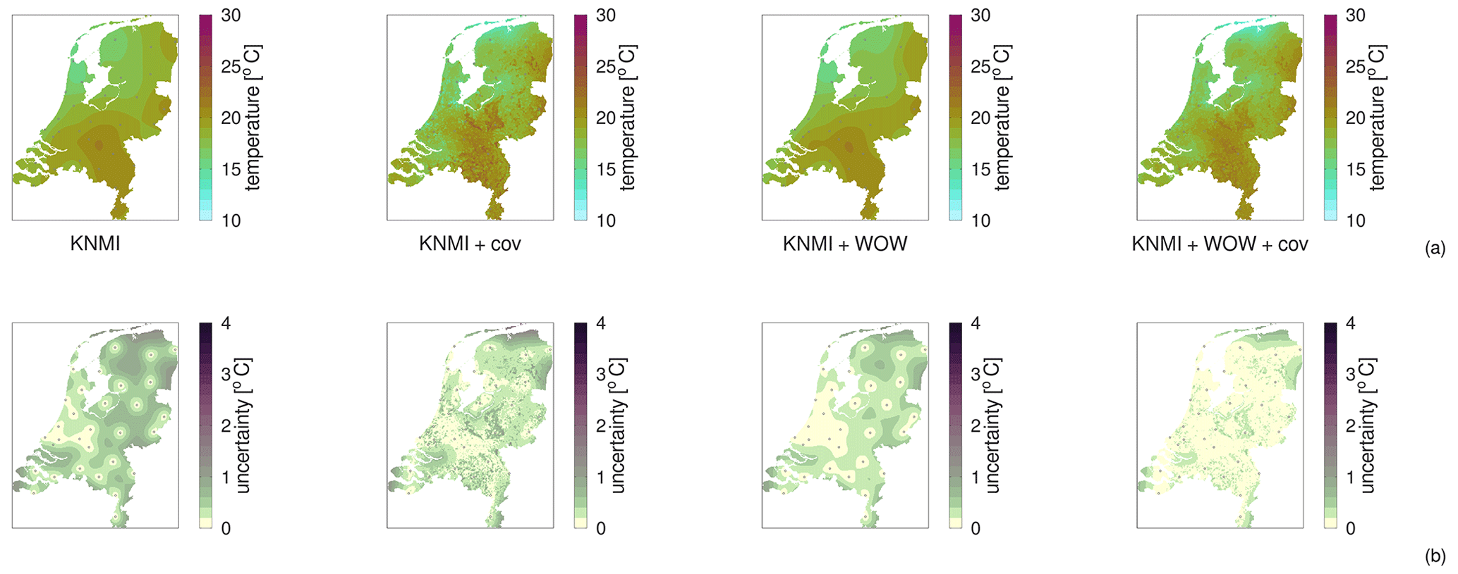
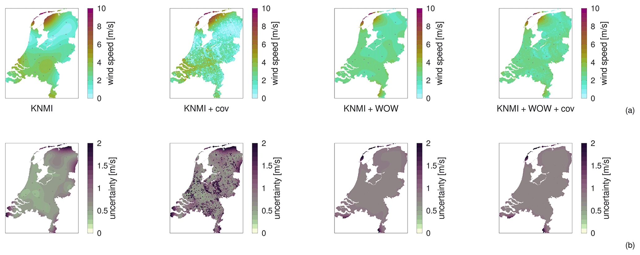
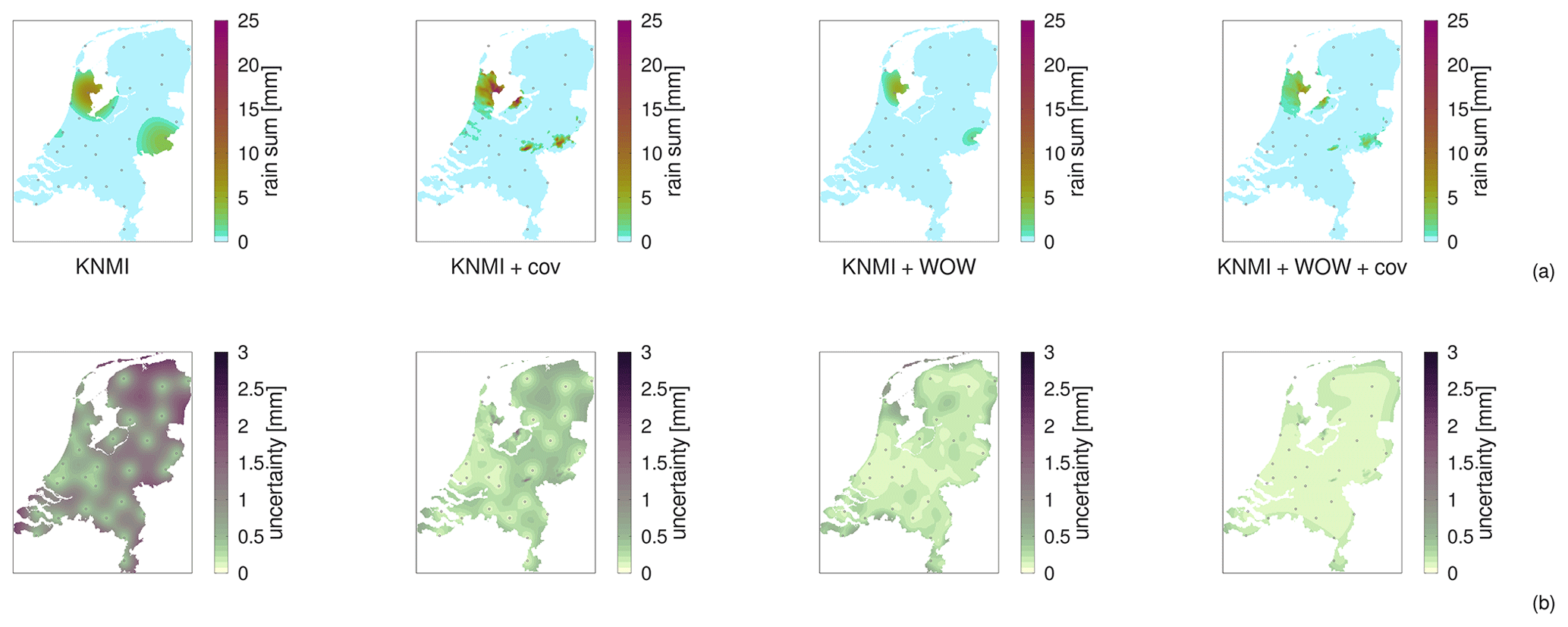
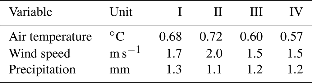
High-resolution weather maps are fundamental components of early warning systems, since they enable the (near) real-time tracking of extreme weather events. In this context, crowd-sourced weather networks producing low-fidelity observations are often the only type of data available at local (e.g. neighborhood) scales. In this work, we demonstrate that we can provide such maps by combining high-fidelity official weather data with low-fidelity crowd-sourced weather data and high-resolution covariate information. Because the crowd-sourced data contains significant bias and noise, we develop an approach to include a bias budget and noise budget in the multi-fidelity Bayesian spatial data analysis. The weights of the different components of these bias and noise budgets are tuned to the data set. We apply this approach to 24 hours of weather data in the Netherlands, for a day that had a “code orange” (i.e. “be prepared for extreme weather with high risk of impact”) weather warning for heavy precipitation. From our analysis, we see a significant – qualitative and quantitative – synergy effect when introducing low-fidelity data and high-resolution covariate information.

1 Data

For 29 June 2021, the KNMI issued a “code orange” weather warning for heavy precipitation in two provinces (i.e. Noord-Holland and Gelderland). We collect the official high-fidelity observations (N=32) from the KNMI network (i.e. 08:00 to 08:00 LT – local time – CET the day next), and the low-fidelity observations (N≈650) from personal weather stations (Kirk et al., 2021) from the WOW-NL network (https://wow.knmi.nl/, last access: 30 May 2023). We also utilize high-resolution covariates (CBS, 2023), such as distance to coast, population, tree cover and rain radar (https://data.4tu.nl/articles/_/12675278/1, last access: 16 December 2022). The rationale is that, for example for wind speed, we expect a local effect on wind speed in areas with high percentage of tree cover, proximity of open water, etc.

2 Methodology

In the context of Bayesian spatial data analysis (Wikle and Berliner, 2007) for producing high-resolution maps (de Baar and Garcia-Marti, 2022; van Beekvelt, 2022), we are interested in predicting m grid values X of an individual variable, conditional on n observations y. In the presence of covariates, we have the prior

$$\begin{array}{}\text{(1)}& p\left(\mathit{X}\right)=\mathcal{N}\left(\mathbf{Q}{\widehat{\mathit{\beta }}}_Q,\mathbf{P}\right),\end{array}$$

where the m×m matrix P is the process covariance matrix (Sect. 2.3, Wikle and Berliner, 2007 and Eq. 3, Hengl et al., 2007). We use a Gaussian kernel to model the prior covariance matrix ${\mathbf{P}}_{ij}={\widehat{\mathit{\sigma }}}_x^{\mathrm{2}}\exp \left(-\frac{\mathrm{1}}{\mathrm{2}}{h}_{ij}^{\mathrm{2}}{\widehat{\mathit{\theta }}}^{-\mathrm{2}}\right)$, with ${\widehat{\mathit{\sigma }}}_x^{\mathrm{2}}$ the estimated process variance and lag h_ij the spatial distance between locations i and j. The correlation length scale $\widehat{\mathit{\theta }}$ remains to be estimated. The m×q matrix Q contains the q covariates evaluated at the grid points, where we use the rain radar as a covariate for precipitation, and distance to coast, population and tree cover as covariates for temperature and wind speed. The q×1 covariate weight vector ${\widehat{\mathit{\beta }}}_Q$ remains to be estimated. The possibility of using a non-Euclidian lag is explored in de Baar and Garcia-Marti (2022) and references therein.

Figure 1 Example grid for hourly mean air temperature, showing (a) predicted mean and (b) predicted standard deviation.

Figure 2 Example grid for hourly mean wind speed, showing (a) predicted mean and (b) predicted standard deviation.

The likelihood is interpreted as a model of the observational process (de Baar et al., 2014; Sect. 2.3, Wikle and Berliner, 2007)

$$\begin{array}{}\text{(2)}& p\left(\mathit{Y}\right|\mathit{x})=\mathcal{N}(H\mathit{x}+B{\widehat{\mathit{\beta }}}_B,R),\end{array}$$

with H the n×m observation operator and B the m×b bias budget matrix containing b bias proxies evaluated at the observation locations. For the n×n noise covariance matrix, we assume spatially uncorrelated noise $\sqrt{R}=N{\widehat{\mathit{\beta }}}_N{I}_{n\times n}$, with N the n×p noise budget matrix containing p noise proxies evaluated at the observation locations. The b×1 bias weight vector ${\widehat{\mathit{\beta }}}_B$ and the p×1 noise weight vector ${\widehat{\mathit{\beta }}}_N$ remain to be estimated. Our rationale is that the – calibrated – high-fidelity observational process includes no bias and only limited uniform noise, while the low-fidelity observational process involves significant bias and noise budgets.

Figure 3 Example grid for an hourly sum of precipitation, showing (a) predicted mean and (b) predicted standard deviation.

The novelty in this approach is that we define a bias budget and noise budget as part of the likelihood. Currently, the bias and noise budgets contain indicators for network type, but they could also include variable members like local population density, local sky view factor, station height above ground, etc. We then estimate the weights of the members of these budgets from the data y. In particular, we estimate the hyperparameters ${\widehat{\mathit{\sigma }}}_x$ ${\widehat{\mathit{\beta }}}_Q$ and ${\widehat{\mathit{\beta }}}_B$ from an analytical maximum likelihood estimate (Hengl et al., 2007, Eq. 4), where we use the same approach for each individual weather variable. For the reason of robustness, we have opted to estimate the hyperparamters $\widehat{\mathit{\theta }}$ and ${\widehat{\mathit{\beta }}}_N$ from brute-force iterative leave-one-out cross-validation (James et al., 2013, Sect. 5.1), where, because of the bias in the low-fidelity data, we only leave out high-fidelity data during cross-validation. The resulting map, which is the result of the above Bayesian updating process, is then a conditional multivariate normal distribution $p\left(\mathit{X}\right|\mathit{y})=\mathcal{N}(\widehat{\mathit{x}},\widehat{C})$, defined by the posterior mean $\widehat{\mathit{x}}=\mathrm{E}\left(\mathit{X}\right|\mathit{y})$ and posterior covariance $\widehat{C}=\mathrm{cov}\left(\mathit{X}\right|\mathit{y})$, which are given by Hengl et al. (2007, Eqs. 5–6) and Wikle and Berliner (2007, Eqs. 5–7). In the posterior covariance, we take into account the uncertainty caused by the use of covariates (Hengl et al., 2007) and apply an inflation factor $f=n/(n-n_{\mathrm{hyp}})$ to account for the observation-based estimation of n_hyp hyperparameters.

3 Results and discussion

Figures 1–3 illustrate weather maps for 08:00–09:00 LT (CET). Here we show results for air temperature, wind speed and precipitation. Each figure shows (column 1) the maps based only on high-fidelity, (column 2) the maps based on high-fidelity and covariate data (column 3) the maps based on high- and low-fidelity, and (column 4) the maps based on high-fidelity, low-fidelity and covariate data. To demonstrate the general applicability of the methodology, we do not presently apply any transformations to the different variables; although this would be possible to do in the future.

In order to quantify the improvement achieved by including additional data, in the following sub-sections we use the terminology by Roache (1998). By validation, we mean that we compare the output of a computer code to observations that were not included as an input. By verification, we mean that we compare the output of one run of a computer code with a different run of the same code, but with different inputs or settings.

3.1 Cross-validation

We apply leave-one-out cross-validation of the high-fidelity KNMI stations to compute a root-mean-squared (RMS) prediction error (James et al., 2013). For robustness, we leave out the lowest and highest error before we compute the RMS prediction error. We repeat this for each of the 24 hourly time slices, and compute an overall RMS error. The results are summarized in Table 1.

Table 1 Leave-one-out cross-validation RMS prediction errors for different variables, using (I) KNMI stations only; (II) KNMI and covariates; (III) KNMI and WOW; and (IV) KNMI, WOW and covariates.

For air temperature and wind speed, we observe overfitting in method II (KNMI + cov), while method IV (KNMI + WOW + cov) gives a slight improvement. For precipitation, we see that method II already gives a good result, which is an indication that the rain radar is a very good covariate for precipitation by itself, even without including WOW data.

3.2 Verification and synergy effect

We have shown that high-resolution, high-confidence maps can be produced by combining high-fidelity data with a dense network of low-fidelity data and suitable covariates. However, the cross-validation in Sect. 3.1 is somewhat biased towards the “ideal” locations of the KNMI stations, which do not sample urban areas and forests, and do not always sample the locations of extreme precipitation. Therefore, from cross-validation we might not observe the improvement of the maps in those areas. To address this issue, in this subsection we run a verification study to quantify the improvement of the entire map, as achieved by including WOW data and/or covariates.

Figure 4 Observed coefficients in a grid RMS difference sensitivity study for 24 individual hours of hourly precipitation sum. The figures show (a) the time series and (b) the same data but now represented in a scatter plot. Negative values indicate that adding data improves the map. “kstation” we indicate 1000 stations.

While in the cross-validation in Sect. 3.1 we used left-out observations as a reference for the output of our spatial regression, in the verification study in this sub-section we use a reference map to compare with. For each hour, we build this reference map by including all available data. Then, we run the spatial regression with a reduced number of WOW stations and/or a reduced number of covariates. Comparing these “reduced data” maps with the reference map provides us with an RMS difference for the entire country. The change in this RMS difference that we observe when increasing the amount of WOW stations and/or covariates gives us an idea of their contribution to the spatial regression output.

In Fig. 4a, we show the effect of including WOW data and/or covariates over time, while in Fig. 4b we show the same data in a scatter plot. Interestingly, we see a “synergy” effect, where adding WOW data and covariates at the same time gives a larger improvement than the sum of the individual improvements. The most likely reason for this is that, by adding crowd-sourced WOW stations, we are not only increasing spatial station density, but are also sampling the higher-value areas (e.g. cities, forests, rain showers) of covariates that we were not sampling before.

References

CBS: Geografische data, https://www.cbs.nl/nl-nl/dossier/nederland-regionaal/geografische-data/ (last access: January 2023), 2023. a
Crameri, F.: Scientific colour maps, Zenodo [code], https://doi.org/10.5281/zenodo.5501399, 2018.
de Baar, J. H. S. and Garcia-Marti, I.: Recent improvements in spatial regression of climate data, in: NATO-AVT-354 workshop on multi-fidelity methods for military vehicle design, 26–28 September 2022, Varna, Bulgaria, https://doi.org/10.13140/RG.2.2.25417.52325, 2022. a, b
de Baar, J. H. S. and Garcia-Marti, I.: Dataset associated to the project “Spatial regression of multi-fidelity meteorological observations using a proxy-based measurement error model”, Version 1, 4TU.ResearchData [code and data set], https://doi.org/10.4121/ffa71bf6-b605-4719-acb5-83b733208e4b, 2023. a
de Baar, J. H. S., Percin, M., Dwight, R. P., van Oudheusden, B. W., and Bijl, H.: Kriging regression of PIV data using a local error estimate, Exp. Fluids, 55, 1650, https://doi.org/10.1007/s00348-013-1650-z, 2014. a
Hengl, T., Heuvelink, G. B., and Rossiter, D. G.: About regression-kriging: From equations to case studies, Comput. Geosci., 33, 1301–1315, https://doi.org/10.1016/j.cageo.2007.05.001, 2007. a, b, c, d
James, G., Witten, D., Hastie, T., and Tibshirani, R.: An introduction to statistical learning, Springer, New York, ISBN 13:978-1461471370, 2013. a, b
Kirk, P. J., Clark, M. R., and Creed, E.: Weather observations website., Weather, 76, 47–49, https://doi.org/10.1002/wea.3856, 2021.  a, b
KNMI: SYNOP – hourly unvalidated observations from the KNMI automated network in text format, https://dataplatform.knmi.nl/dataset/ (last access: 2 June 2023), 2023a. a
KNMI: WOW-NL: Jouw weer op de kaart! – KNMI, https://wow.knmi.nl/ (last access: 2 June 2023), 2023b. a
Overeem, A. and Imhoff, R.: Archived 5-min rainfall accumulations from a radar dataset for the Netherlands, Version 1, 4TU.ResearchData [data set], https://doi.org/10.4121/uuid:05a7abc4-8f74-43f4-b8b1-7ed7f5629a01, 2020. a
Roache, P. J.: Verification and validation in computational science and engineering, Hermosa, Albuquerque, NM, ISBN 13:978-0913478080, 1998. a
van Beekvelt, D.: Multi-fidelity spatial regression for air temperature predictions using first, second and third party data, MSc thesis, Utrecht University, Utrecht, https://studenttheses.uu.nl/handle/20.500.12932/43339 (last access: 26 May 2023), 2022. a
Wikle, C. K. and Berliner, L. M.: A Bayesian tutorial for data assimilation, Physica D, 230, 1–16, https://doi.org/10.1016/j.physd.2006.09.017, 2007. a, b, c, d
Download
Short summary
Combining high-fidelity official meteorological observations with low-fidelity crowd-sourced data in a single climate or weather map is challenging because of the significant bias and noise in the low-fidelity data. In this work, we present a method to treat this bias and noise in a statistical framework. In addition, we show that we can make an additional improvement in the quality of the map when we add high-resolution land use information.