Internal boundary layer characteristics at the southern Bulgarian Black Sea coast

The marine Atmospheric Boundary Layer (ABL) over the southern Bulgarian Black Sea coast is studied based on remote sensing measurements with a monostatic Doppler sodar system located at about 400 m inland. Long-term profile data (August 2008–October 2016) with high spatial (10 m) and temporal (20 min running averages at every 10 min) resolution was analysed to reveal the complex vertical structure of the coastal ABL at marine airflow. The processes of air masses transformation due to the sharp change in physical characteristics of the underlying surface lead to Internal Boundary Layer (IBL) formation. Its spatial scales as a sublayer of the coastal ABL depend on the distance from the shore. In the absence of temperature and humidity profile measurements, the turbulent profiles of marine air masses of different fetch over land (400 to 2500 m) were used to examine the characteristics of the IBL. Different fetch or distance passed by the marine airflow before reaching the sodar is considered selecting intervals of wind directions. IBL heights between 60 and 150 m depending on the fetch are obtained.

1 Introduction

The importance of the ABL studies is essential because we live and work in it. Changes in the structure and dynamics of the ABL have a direct impact on most human activities which are mainly concentrated in this bottom layer of the atmosphere. The ABL characteristics are directly affected by the properties of the Earth's surface (Stull, 1988) and its abrupt change (such as field-city, sea-land, field-forest, etc.) leads to a complex ABL layering due to the transformation of the air masses to the physical characteristics of the new surface. The IBL height depends on the distance from the shore (Batchvarova et al., 1999). During summer days, the transformation of the cooler and moist marine air over heated land leads to the formation of a Convective Internal Boundary Layer (CIBL), with height depending on air temperature, wind speed, turbulent exchange, and atmospheric stability and the process of marine air masses transformation over the new surface (Hsu, 1986; Garratt, 1990; Melas and Kambezidis, 1992; Batchvarova et al., 1999). The marine air located above the CIBL is stably stratified and it limits the volume to which air pollutants can spread. The CIBL is very shallow close to the shore and the pollutant emissions within it lead to their accumulation (Simpson, 2007). In addition, the unfavorable impact on the air quality increases with the presence of closed local circulation.

Such complex and dynamic interactions are challenging for numerical weather prediction (NWP) and air quality models. The ABL parameterization schemes used in the weather, climate, and pollutant dispersion models are a key element for the determination of the small-scale turbulent fluxes, vertical diffusion and for the proper prediction of the near-surface meteorological parameters with a high spatial and temporal resolution (Anurose and Subrahamanyam, 2015). The ABL parameterization schemes are usually designed and tested for flat homogeneous terrain. Their improvements to complex surfaces contribute to the enhancement of the NWP models. Therefore, studying the characteristics and dynamics of the coastal IBL by conducting detailed and long-term meteorological measurements in such areas is of great importance for weather and climate forecasts, air quality management and, respectively, human health protection.

Over the past decade, the advanced ground-based ABL profiling has been used by a number of studies as a reliable method for detailed understanding and improvements of the theoretical descriptions of the atmospheric processes, and also for evaluation of numerical models (Floors et al., 2013; Gryning et al., 2014; Salvador et al., 2016; Lyulyukin et al., 2019; Lo Feudo et al., 2020). The technological advancement of this type of remote sensing instruments led to their widespread use and to the realization of a number of cooperation projects in the field of science and technology under the European COST program with several Actions as COST Action ES0702 (EGCLIMET), COST Action 720, COST Action ES1303, (TOPROF) and COST Action CA18235 (PROBE) (Engelbart et al., 2009; Illingworth et al., 2013, 2015; Cimini et al., 2020). The interdisciplinary studies and cooperation within all these research networks are of great importance for improving weather forecasting and increasing the quality of all meteorological products at the service of society by integrating a number of ground-based instruments for ABL profiling into a European observation network.

The presented study here is based on long-term acoustic soundings data for the coastal atmosphere with a high temporal and vertical resolution of the profiles of standard meteorological parameters and turbulence characteristics. The derived results are unique for Bulgaria, where the ground-based remote sensing measurements are not widely used in operational mode.

2 Study area, measurements and methods

2.1 Area and equipment

Meteorological Observatory (MO) Ahtopol is the southernmost synoptic coastal station of the operational network of the Bulgarian National Meteorological Service located about 2 km in the southeast direction from the town of Ahtopol in south-eastern Bulgaria (Fig. 1). The south-eastern Bulgarian coastline has an approximate northwest-southeast direction without significant incisions in the land, except for Burgas Bay which is the largest one in Bulgaria. The study region falls in the Black Sea climatic sub-region of the Mediterranean climatic region characterized by mild winters, breezy summers, and smoothly occurring transit seasons (Barantiev et al., 2021). The terrain of MO Ahtopol is flat and grassy located about 400 m inland. The shore rocks are about 10 m high. The instrument used is a multi-frequency mono-static Doppler remote sensing system installed on the roof of the administrative building (at a height of 4.5 m) (Fig. 1 – right). The operating frequency range of the multi-beam sodar (SCINTEC MFAS model) is 1650–2750 Hz with 9 emission/reception angles (0, ±9.3, ±15.6, ±22.1, and ±29^∘), first measurements level at 30 m, a vertical resolution of 10 m up to 1000 m (Scintec AG, 2018).

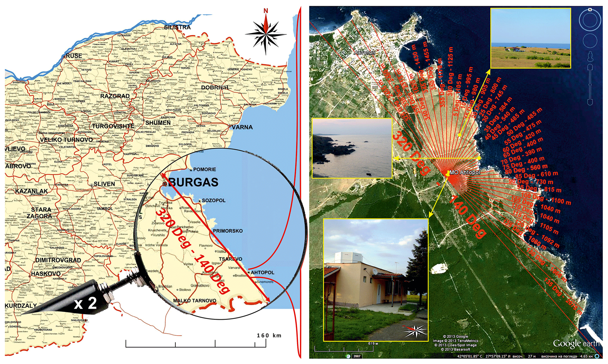
Figure 1 Location of MO Ahtopol and the coastline stretch direction in the southeastern part of the Bulgarian Black Sea Coast (left panel) (Newebcreations), and a satellite image (© Google Earth) of the study area with the distances in meters to the sodar from the coast line, calculated every 5^∘ of change in the geographical direction from 320 to 140^∘ and authors' personal photos from the area (right panel).

Although the MFAS always provides results in the best possible height resolution (10 m steps), the effective height resolution is often larger depending on the acoustic pulse lengths. The acoustic pulse lengths are set to vary from 10 m for the first few measurement levels up to 50 m above measurement levels corresponding to 100 m height to improve the backscattered signal-to-noise ratio (SNR). All the turbulence-related quantities presented in this are sodar probe volume and beam frequency dependent.

2.2 Data and methods

Accumulation and study of the acoustic remote sensing data at the Bulgarian coast began in the summer of 2008 in MO Ahtopol under a scientific collaboration between the National Institute of Meteorology and Hydrology at the Bulgarian Academy of Sciences (NIMH – BAS) and Research and Production Association (RPA) “Typhoon” – Russian Federal Service for Hydrometeorology and Environmental Monitoring (Roshydromet). This joint project laid the foundations of ABL climate studies with high spatial (every 10 m) and temporal (output data every 10 min with 20 min averaging) resolution (Barantiev et al., 2011; Novitsky et al., 2012). The acoustic measurements in MO Ahtopol taken into account in this study cover a period from the beginning of August 2008 to the end of October 2016. A total of 341 971 profiles were analyzed in this study, corresponding to 78.8 % temporal coverage of the 3014 d period. The full information on the spatial and temporal data availability of that acoustic database is presented in Barantiev et al. (2021).

The marine ABL characteristics in this study are presented by averaged profiles of 12 output sodar parameters and their dispersions – wind direction (WD), wind speed profile (WS), WS dispersion (sigWS), vertical wind speed (W), W dispersion (sigW), horizontal (western) component of the WS profile (U), U dispersion (sigU), horizontal (southern) component of the WS profile (V), V dispersion (sigV), eddy dissipation rate (EDR), turbulent intensity (TI) and turbulent kinetic energy (TKE). The detailed information on the sodar output parameters calculations given in Scintec AG (2017) is based on theoretical descriptions of Monin and Yaglom (1971) and studies of Kouznetsov (2000) and Kramar and Kouznetsov (2002). The thermodynamic state of the marine ABL is studied by sodar output of the atmospheric stability classes according to the Pasquill-Gifford classification using the σ_ϕ method (Bailey, 2000) and in addition by Buoyancy Production (BP) profiles which are calculated using sigW (σ_w) output derived from sodar at different altitudes (z) with Eq. (1) (Engelbart et al., 2009):

$$\begin{array}{}\text{(1)}& \mathit{\beta }={\displaystyle \frac{{\mathit{\sigma }}_w^{\mathrm{3}}}{z}},\end{array}$$

Representative averaged profiles from the sodar output for different lengths of the marine air masses run over land are used to check whether the formation of IBL can be observed in the sodar data. The method suggested by Illingworth et al. (2013, 2015) for ABL height estimation based on turbulence profiles is used. A satellite photo of the area of MO Ahtopol is shown in Fig. 1 (right – © Google Earth picture), on which distances in meters from various points of the coastline to the location of the sodar (administrative building), are graphed. The fetch is estimated as follows:

• short fetch: from 35 to 80^∘ – marine air masses run from 390 to 584 m above the land;

• middle fetch: from 355 to 15^∘ and from 100 to 125^∘ – run from 980 to 1170 m above the land;

• long fetch: from 325 to 350^∘ and from 130 to 135^∘ – run from 1430 to 2480 m;

To eliminate the presence of many short profiles, additional conditions are imposed: at least 10 points with measurements in height; the first point of profile to fall within respective wind-direction intervals of the fetches; the height of the profile is determined by the fulfillment of the wind-direction conditions; breaks in the profile are allowed only due to a lack of data.

3 Results

3.1 Average characteristics

In remote sensing measurements, there may be altitudes from which data are not received or rejected by signal quality algorithms. In the case of Doppler lidars, the presence of aerosols in the atmosphere is necessary for the continuous availability of data in the profiles, and for the sodars, the presence of temperature/turbulent inhomogeneities is needed. A comparison of the performance and the evaluation of the measured wind profiles of these two remote sensing instruments are presented in Torres Junior et al. (2022). The nature of acoustic soundings of the atmosphere lead to different data availability in the derived averaged sodar profiles at different altitudes (spatial inhomogeneity). This leads to averaged characteristics formed by a different number of measurements at the respective heights. The highest availability of sodar data (over 90 %) is observed up to a height of 190 m (Barantiev et al., 2021). The average profile presented in this study might be biased compared to eventual continuous measurements at all vertical levels. In this study, the tracking of changes in the averaged profiles is carried out only qualitatively, not quantitatively, and each of the presented analyses is individual for the specific case and cannot be unified with exact values or statements.

3.1.1 Short fetch

The values of the averaged vertical profiles (colored dots) of the marine air masses and their dispersions (green areas) derived from up to 7915 profiles (2.3 % from all measurements) satisfying the condition of WD from 35 to 80^∘ are presented in Fig. 2. The color of the dots denotes the number of profiles involved in the output of the averaged characteristic at a certain height and it is indicated through the color bar on the right side of the graphs. The turbulent profiles of sigWS, sigU, sigV, and TI have the lowest profiles availability since they are calculated as a second statistical moment and the sodar signal quality algorithms have stronger weight on these variables. These marine air masses have the shortest fetch (from 390 to 584 m). The average characteristics in Fig. 2 represent superposition of mesometeorological and local forcing in the area since no additional conditions have been placed. The changes observed in the vertical gradients of the averaged profiles of WS, W, U, V, and EDR, as well as almost unchanged values of the turbulence parameters of sigW, TI, and TKE at a height of 40 m above ground level (a.g.l.) are an indicator of surface layer (SL) height.

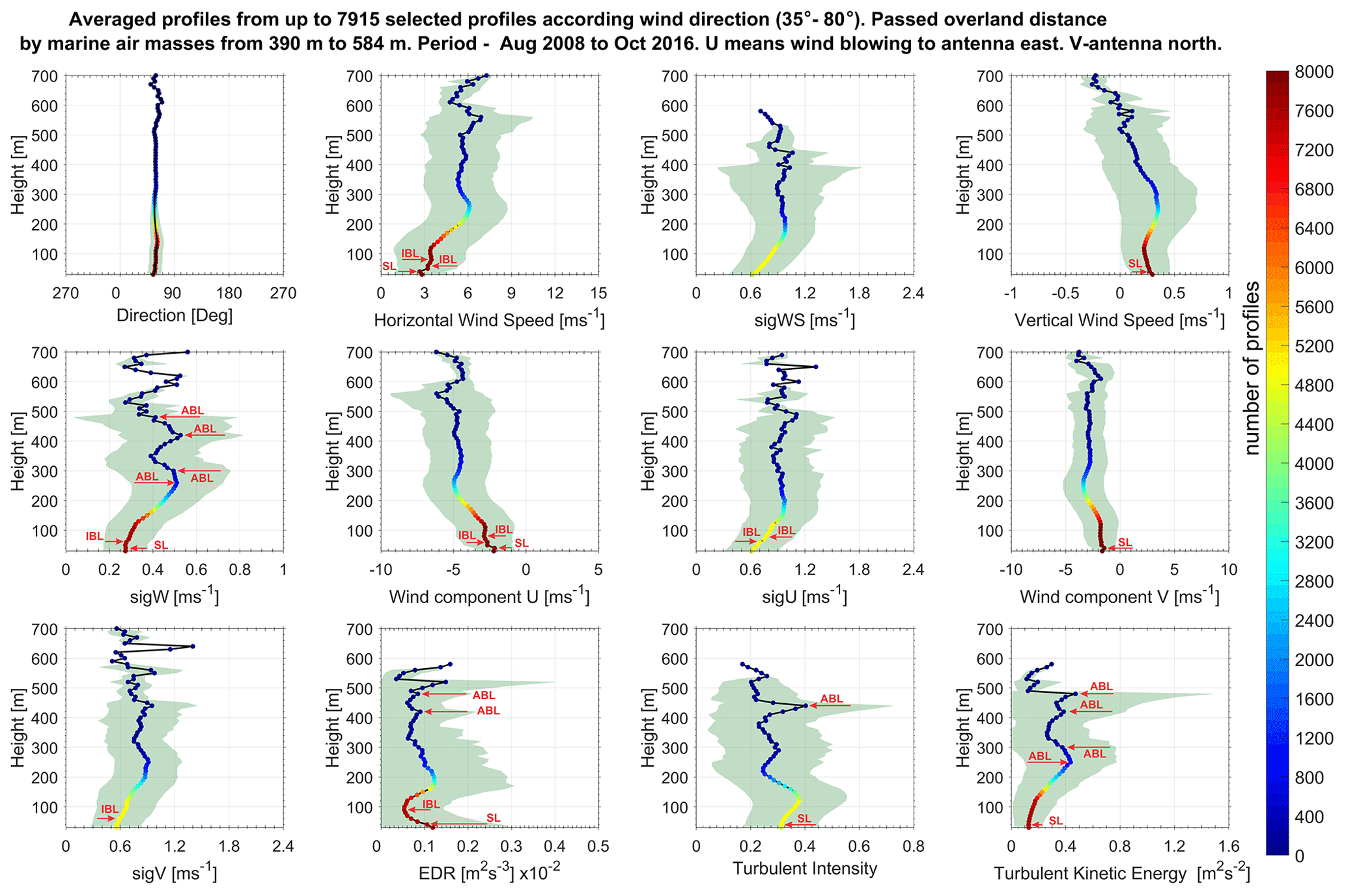
Figure 2 Vertical structure of a coastal ABL (MO Ahtopol) determined from averaged profiles (colour dots) and their dispersions (green area) of 12 output parameters (sodar MFAS – SCINTEC) corresponding to a distance travelled over land by marine air masses from 390 to 584 m. From left to right and top to bottom the parameters shown are: WD, WS, sigWS, W, sigW, U, sigU, V, sigV, EDR, TI. and TKE. The colour legend denotes the number of profiles reaching the specific height.

Tracking the shape of the WS profile near the surface, changes in the vertical gradient at 50, 70, 90, and 120 m are observed. Similar changes but with the opposite sign are observed for the vertical gradient of the U profile at the same altitudes. A slight increase in the values of the vertical gradient of the sigU profile at 50, 70, and 130 m is also observed, and this trend but with smaller values in the gradient changes is also present in sigV. A very small change is observed in the vertical gradient of sigW profile at 70 m and an almost linear increase after this height up to 110 m. Near the surface, the values in the EDR profile decrease rapidly with height up to 70 m and after 90 m the observed negative gradient becomes positive. A pronounced peak is observed at 120–130 m at TI, with the highest vertical gradient between the heights of 60–110 m a.g.l. These changes in the average profiles reveal possible heights of IBL at 60 m a.g.l. and in the range of 80–90 m.

The sigW plot shows a well-defined peak in the profile at a height of 260 m to 300 m a.g.l. At these altitudes, a satisfactory availability of retrieved profiles (from 926 at 260 m to 466 at 300 m) participating in the derivation of the averaged values is observed. Similar changes in the sign of the averaged profile gradient and in its dispersions are observed for one more turbulent parameter at almost the same height (TKE at 250–300 m). At the same height, the values of the WS and W also stop increasing. The changes at 250–300 m could be related to the height of marine ABL, but also the altitudes 250–260 m could be related to the height of the sea breeze cell core where the maximal wind speed is observed during typical for the study area local coastal circulations (Barantiev et al., 2017). The next well-pronounced peak of sigW is observed at 420 m with 42 involved profiles at that altitude. That peak is supported by changes in the sign of the gradients of the averaged profiles of EDR, TI, and TKE almost at the same altitude and can be associated with the marine boundary layer height at 420–440 m a.g.l. High dispersion value and well-pronounced peak are observed in TKE profile at 480 m where 9 individual profiles are involved in the calculation of the averaged value. This altitude could be also assumed as a marine ABL height finding confirmation in observed weaker peaks but again with high dispersion values at sigW and EDR profiles, respectively with 11 and 8 involved profiles. The gradient of the WS profile sharply changes its sign from negative to positive at 610 m, and at 620 m, a third pronounced peak at sigW is observed. These changes could also be associated with the height of the marine ABL, but unfortunately due to the low availability of profiles at this height (6 for WS at 610 m and 2 for sigW at 620 m), no confirmation can be obtained from other averaged profiles.

3.1.2 Middle fetch

Averaged profiles and their dispersions characterizing marine air masses with winds corresponding to travelled distance above the land from 980 to 1170 m (8251 profiles representing 2.4 % from all measurements) are presented in Fig. 3. The high dispersions of the averaged profile of the WD and its values show that the individual profiles that took part in the derivation of the averaged characteristics are distributed almost evenly between the defined “wind windows” (355÷15 and 100÷125^∘) up to 340 m a.g.l., which in turn determines the existence of a superposition in the averaged results between different situations of marine boundary layer over land (nocturnal or diurnal, or such during the cold, or warm half of the year). The main peak in the averaged sigW profile is observed at 280–290 m a.g.l. (respectively 366 and 351 involved profiles at these altitudes), and the second one, which is more pronounced in the dispersion values (green area) at 380–410 m (respectively 41 and 13 involved profiles). Well-pronounced changes from increasing to decreasing values of the averaged EDR and TKE profiles are also observed at 280–310 m. Weak negative peaks in sigW and TKE are observed at 50–60 m a.g.l. EDR values rapidly decrease to a height of 60 m forming a negative peak at 90 m. The TI profile decreases its values from 30 to 70 m and begins to increase to a pronounced peak at an altitude of 130–160 m. In the values of the averaged profile of the WS, a slightly pronounced peak is observed at a height of 80–90 m, and after 120 m a very weak positive peak at 150 m. The changes in this profile are continued with a slight increase in the values up to 240 m, followed by almost unchanged values up to 390 m and more sharp changes after 420 m. In the averaged profile of W, a smooth decrease in values is observed, and more frequent changes in the vertical gradient begin to be observed after 410 m (67 involved profiles). The averaged profiles of sigW, EDR and TKE have higher values in the first 150 m a.g.l. compared to the same parameters plotted in Fig. 2, with the most significant difference observed in the lowest parts of the EDR profiles. In the profile of the WS and its components, characteristic changes are again observed at 40 m determining the height of the SL. For IBL height could be pointed in the range of 60–90 m (sigW, EDR, TKE, TI, WS). The observed changes in presented turbulent profiles have revealed marine boundary layer height at 280–310 m (sigW, EDR, TKE). Another height that can be associated with that of the marine boundary layer is 380–410 m (sigW, WS, W). The breeze characteristics are revealed with the height of the sea breeze core at 130–160 m (WS, TI).

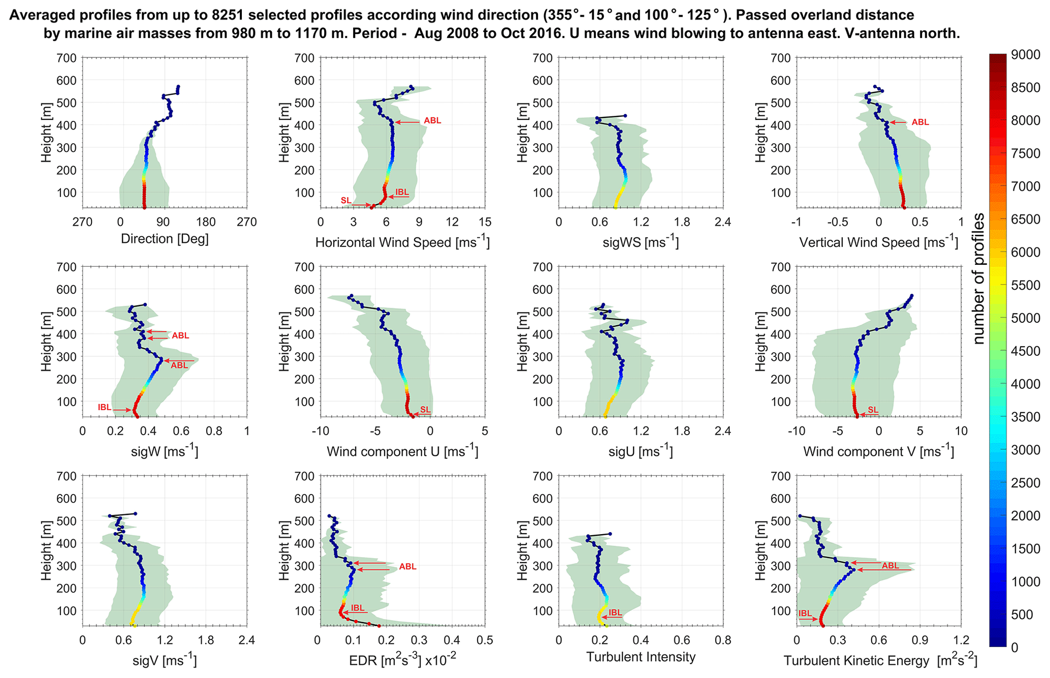
Figure 3 Vertical structure of a coastal ABL corresponding to a distance travelled over land by marine air masses from 980 to 1170 m. Details as in Fig. 2.

3.1.3 Long fetch

The lowest availability of involved profiles in the performed statistical analysis of marine air masses is observed for WD condition corresponding to the long fetch. The averaged characteristics of that most strongly influenced marine flow (1430–2480 m over land) are derived from total 4801 profiles (1.4 % from all measurements) and are presented in Fig. 4. The lowest availability of involved profiles is partly due to the smallest wind direction “windows” (lack of involved profiles from the southeast WD – Fig. 4). This, in turn, affects the maximum height reached by the presented 12 averaged profile characteristics. For the profiles calculated as a second statistical moment (those with the lowest availability) the maximum height reached is 420 m. A check of the number of profiles involved up to a certain height shows that the average value of sigWS profile at a height of 400 m is calculated from the values of only two profiles. This is also the case when deriving the mean values of EDR at a height of 450 m. After these heights, no averaging is actually done, and the derived values are based on one profile only (respectively without dispersion area).

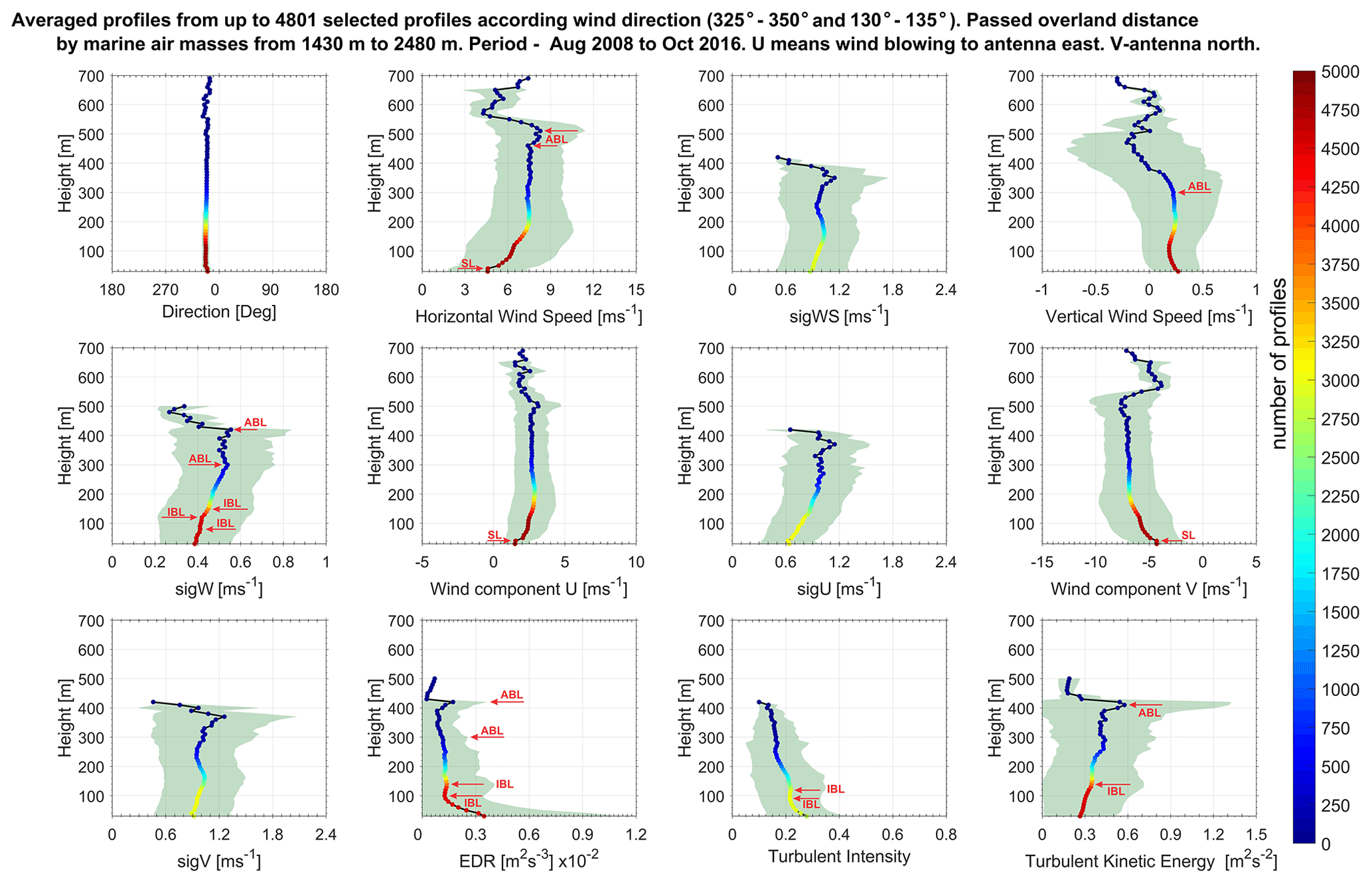
Figure 4 Vertical structure of a coastal ABL corresponding to a distance travelled over land by marine air masses from 1430 to 2480 m. Details as in Fig. 2.

Almost unchanged values of averaged profiles of WS and the horizontal wind component (U and V) up to 40 m a.g.l. are observed and related with the SL height. After the SL the shape of the WS profile changes almost parabolically up to 120 m, followed by a weakly pronounced peak at 270–290 m and almost no changing values up to 460 m (36 profiles available). A well-pronounced peak in this profile is observed at 510 m (10 profiles available) followed by sharp drop in values by about 4 m s⁻¹ at 570 m (5 profiles available). Positive values of W are mainly observed up to 370 m, as the first negative peak in this profile is observed at 100 m, and after 300 m the average values start to decrease more sharply. The average profile of sigW increases up to 300 m with visible changes in its vertical gradient and dispersion values at 40, 80, 120, and 150 m. A significant change in the values of this profile is observed at 420 m where only 6 profiles are involved in the calculation lowering their count to 2 after that height. EDR average profile sharply decreases up to 100 m, forming different gradient changes after that (more visible at desertion values) at 140, 250, 300, and 420 m. The TI profile generally decreases its values in height forming two weak negative peaks at 90 and 250 m and one weak positive at 120 m. The mean values of this profile have the lowest values compared to those shown in Figs. 2 and 3. The averaged values in the TKE profile increase in height up to 410 m, where the most pronounced positive peak is found, followed by a sharp decrease in the values. Weaker changes in the gradient of the averaged TKE profile are observed at 140–150, 260, and 290 m. The observed changes in the presented profiles in Fig. 4 have revealed 40 m SL height (WS, U, and V) and 300 m marine boundary layer height (W, sigW, and EDR). Other heights that can be associated with that of the marine boundary layer are 410–420 m (sigW, EDR, and TKE) and 460–510 m (WS) indicating the size of the shallow sea breeze cells falling within the range of the sodar (Barantiev et al., 2011; Kirova et al., 2018). For IBL height could be pointed in the range of 80–100 m (W, sigW, EDR, TI,) and 120–150 m (WS, sigW, EDR, TI, TKE). The breeze characteristics are revealed with the height of the sea breeze core at 250–260 m (EDR, TI, TKE) and 270–290 (WS, EDR). The highest averaged values for the WS and also for the turbulent profiles of sigW, EDR and TKE are observed at the longest interaction between the marine air masses and the land, comparing the results presented so far (Figs. 2, 3 and 4).

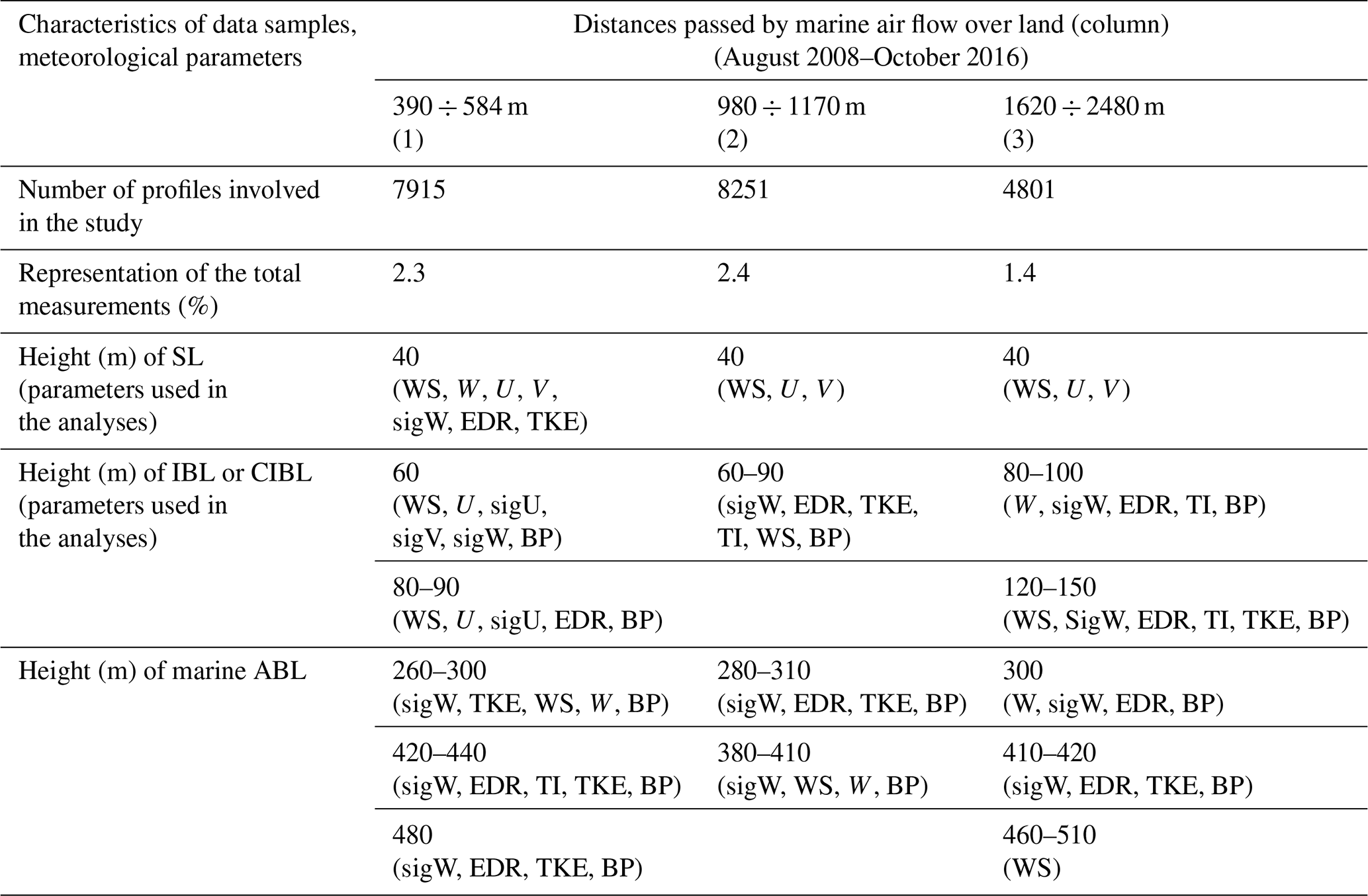
The main results from this climatological study are summarised in Table 1. The identified peaks in turbulence characteristics profiles show surface layer (SL) height of about 40 m, IBL height of 60 m at the short fetch, 90 m at middle and up to 150 m at the longest fetch. The marine ABL height was estimated to about 400 m.

Table 1 Marine boundary layer and analysis over an 8-year measurement period.

3.2 Thermodynamic state

Averaged profiles and their dispersions of Buoyancy parameter derived from individual profiles calculated by Eq. (1) are presented in Fig. 5 for the three different cases of the path travelled over land by marine air masses. The presented results of the three graphs are in agreement with the changes in the shape of the averaged profiles of the turbulent parameters sigW, EDR and TKE presented in Figs. 2, 3 and 4 and largely confirm the deduced heights of the marine ABL and IBL so far. Higher values are also obtained in the BP profiles at the longest passed distances over land as sharp decreases in the values of all presented profiles are observed rising in height and moving away from the influence of the ground where the turbulent heat flow is maximum.

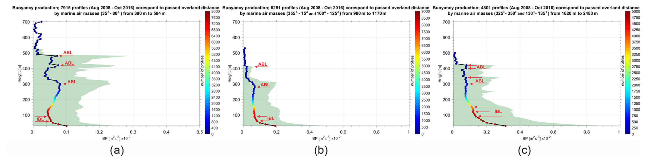
Figure 5 Averaged profiles of Buoyancy parameter corresponding to different fetch of the marine air masses – (a) from 390 to 584 m, (b) from 980 to 1170 m and (c) from 1620 to 2480 m. The colour legend denotes the number of involved profiles reaching the specific height.

A significant change in the gradient of the BP profile of the short fetch (Fig. 5a) occurs after 60 m height where the averaged values start to decrease almost linearly in height up to 90 m forming a negative peak up to 110 m. These changes can be associated with the characteristics of IBL. The determined possible heights of the marine ABL in this case (analyses from Fig. 2) are supported through well expressed positive peaks in the averaged values of the BP profile and its variances at 300 m, 420 m, and 480 m a.g.l. (Fig. 5a).

Almost two times higher values are obtained in the averaged BP profile at middle fetch (Fig. 5b) compared to the short one (Fig. 5a). The observed changes in the shape of the BP profile close to the surface in Fig. 5b are similar to these observed in Fig. 5a but the obtained shape of the averaged profile (Fig. 5b) has a smoother change at 60 m followed again by almost linear variations up to 90 m determining the IBL vertical dimension. After this height, weak changes are obtained in the averaged values of the profile until a positive peak is formed at 280 m and less pronounced at 410 m (Fig. 5b). These heights confirm the heights of marine ABL determined at middle-passed distance (analyses from Fig. 3).

The highest values of the Buoyancy parameter are derived for the long fetch (Fig. 5). The deduced heights of the IBL from Fig. 4 are confirmed by observed changes in the BP profile shape (Fig. 5c). Close to the ground up to 90 m the vertical gradient has high values, then up to 120 m it keeps its negative sign, and the averaged values are changed almost linearly. This is followed by a brief change in the sign of the vertical gradient to a positive value at 130 m and again an almost linear and evenly decrease in values until 150 m. The deduced heights of the marine ABL are confirmed by BP profile form Fig. 5c with a weak peak of the averaged profile at 300–340 m and a second one at 400–430 m. These two peaks are more pronounced in the changes of the dispersion values of the BP averaged profile.

More information about the thermodynamic state of the coastal ABL for different fetch of the marine air masses over land is obtained by the sodar output of the atmospheric stability classes according to the Pasquill-Gifford classification (Bailey, 2000). The results are presented through diagrams of stability classes probabilities at different heights shown in Fig. 6. A 100 % probability is obtained by summing all available probabilities values of the atmospheric stability classes at respective altitudes in each diagram in Fig. 6.

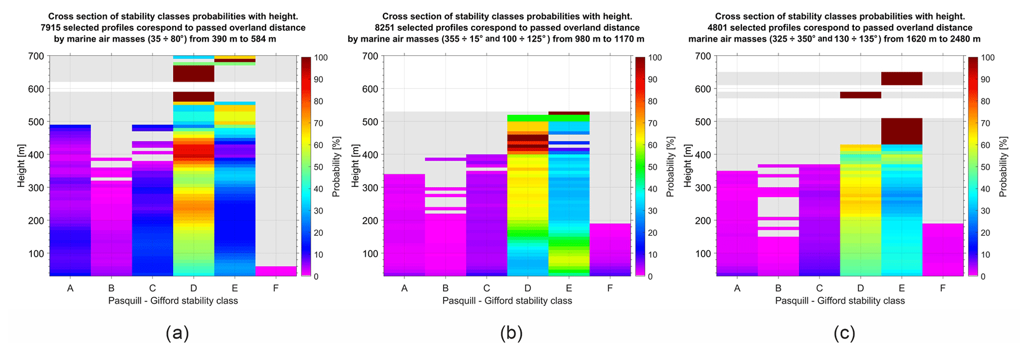
Figure 6 Diagram of stability classes probabilities at different heights corresponding to different distance travelled over land by marine air masses – (a) from 390 to 584 m, (b) from 980 to 1170 m and (c) from 1620 to 2480 m.

For the short fetch (Fig. 6a) the neutral atmospheric stratification (D) can be indicated as the dominant class with more than 63 % probability almost throughout the acoustic sounding layer and with 100 % probability in the layer 560–660 m. The next dominant class according to the Pasquill-Gifford classification used is slightly stable (E) with about 24 % of the averaged probability distribution for the whole vertical layer of measurements. The sequence continues with weakly unstable (C), extremely unstable (A), and moderately unstable (B) with respective average values for the entire layer of about 7 %, 5 %, and 1 %. The stable stratification (F) is also registered but with values under 0.3 %.

A more stable stratification of the marine boundary layer is observed in the case of the middle fetch compared to the short one (Fig. 6b, a) but again the first two dominant atmospheric stability classes remain neutral (D) and slightly stable (E). The first one (D) is with about 57 % average probability for the entire measurements layer and a minimal value of about 30 % at 60 m a.g.l. and the second one (E) with 37 % average probability and a minimal value of about 8 % at 410 m a.g.l. (Fig. 6b). About 3 % of an averaged probability is registered as a weakly unstable (C) stability class with a maximum value of about 10 % at the first measurements level at 30 m and a minimum value of about 2 % at 340 m. The descending sequence continues with extremely unstable stratification (A) followed by stable (F) atmospheric stability class both around 1 % average probability for the entire layer and respectively with maximum values of about 7 % at 30 m and about 2 % at 90 m.

The most stable stratification of the marine boundary layer is observed in the diagram of the long fetch of the marine flow over land (Fig. 6c). An exchange of places in the first two dominant classes according to the averaged values of the probability distribution for the entire measurements layer is observed compared to previous diagrams (Fig. 6a, b) due to the dominant presence of 100 % probability after 420 m in slightly stable (E) atmospheric stratification. The slightly stable (E) atmospheric stability has almost 50 % average probability for the entire layer, while the neutral stratification (D) has a 46 % probability. Below 420 m the neutral stratification (D) remains the dominant class with a 67 % average value for the probability distribution with a minimum of 44 % at 390 m versus 56 % average values for the slightly stable (E) stratification with an observed minimum of 27 % at 270 m a.g.l. The extremely unstable (A) stratification is in third place by average probability distribution with more than 1 % and a maximum value of 7 % at 30 m.

4 Conclusions

The study provides estimations of the IBL height for different fetches of marine air flow over land, namely 60 m for the shortest, 90 m for the middle and 150 m for the longest fetch. This is important information for the conditions of air pollution accumulation. The marine ABL height was estimated to be about 400 m. The surface layer depth is about 40 m. Before the sodar observations, only surface data of climate or synoptic stations were available, thus strongly limiting the research only to near-surface conditions. A more stable stratification of the coastal ABL is observed with the longest run of marine air masses over land as these flows are coming from the North and bring cooler air masses. Another important result is that the registered atmospheric stability classes above 400 m a.g.l. are mostly neutral and slightly stable.

The presented statistical analysis is based on reliable long-term acoustic soundings of the coastal ABL with high spatial and temporal resolution. Such data is of great importance for the study and the theoretical description of the atmospheric processes in similar complex terrain regions and can be used for the validation of different NWP and prognostic air pollution models. Such data is critically needed for the development of improved ABL parametrization schemes in order to achieve more reliable results in the numerical simulations of the meteorological processes in coastal zones. The authors are open to share the data for collaborative studies.