Lagrangian model with heat-carrying particles

The dispersion of pollutants in the atmosphere, whether from industrial emissions, wildfires, or other sources, poses significant challenges to air quality management and environmental protection. Understanding the behavior of plumes is crucial for predicting their dispersion patterns and potential impacts on human health and the environment. In this work, we present a new plume rise scheme based on heat transport. The idea at the basis of the new algorithm is the same as the actual scheme embedded in the Lagrangian Particle Model SPRAY-WEB. The temperature difference between the ambient and the plume and the vertical velocity of the plume are expressed on a fixed Eulerian grid. The particles are assigned with an equivalent momentum, temperature, mass, and density, transported as scalar quantities with the particles following the Lagrangian description of the motion. This allows us to reproduce the entrainment phenomenon as a mixing of two fluids (environmental air and plume) with different temperatures: the resulting temperature is given by Richmann's law.

The results obtained with the old plume rise algorithm and the new one are compared with Briggs (1975) analytical curve in the case of an idealized atmosphere with a neutral stratification and a constant horizontal wind and with experimental data. From the comparison in an ideal atmosphere, it emerged that with the new algorithm, the plume reaches a higher height than with the old one and the asymptotic trend obtained with both models follows the Briggs curve. As for the comparison with the measurements, the results obtained with the new algorithm are in better agreement with the experimental data than the old one.

1 Introduction

The computation of plume rise is one of the basic aspects for a correct estimation of the transport and dispersion of airborne pollutants and for the evaluation of ground level concentration. A forced buoyant plume rises under the action of its initial momentum and buoyancy. It experiences a shear force at its perimeter, where momentum is transferred from the plume to the surrounding air, and ambient air is entrained into the plume. This phenomenon, entrainment, is responsible for the plume diameter increase, of the decrease of its mean velocity and of the average temperature difference between air and plume as well. In the first stage the plume also spreads under the action of the buoyancy-generated turbulence but progressively the effect of ambient turbulence becomes predominant. In a calm atmosphere, plumes rise almost vertically, whereas in windy situations they bend over. In this case, the velocity of any plume parcel is the vector composition of horizontal wind velocity and vertical plume velocity in the first stage and then approaches the horizontal wind velocity. In the Eulerian dispersion models, the calculation of plume rise is based on the fluid dynamic equations, namely on the mass, momentum and energy conservation equations. A complete, exhaustive theory is not yet available. These equations are closed using the entrainment assumption proposed by Morton et al. (1956), which prescribes that the entrainment velocity, i.e., the rate at which ambient air is entrained into the plume, is proportional to the mean local rise velocity

In Lagrangian Particle Models (LPMs), plume rise can be dynamically computed, i.e., each particle, at each time step, can respond to local conditions: wind speed and direction, ambient stability and turbulence (both the self-generated and ambient ones). This allows a high degree of resolution to be obtained. Moreover, it allows simulating the interaction of a plume with a capping inversion layer and the mixture of different plumes in a “natural” way. However, introducing the plume rise computation in a LPM is not straightforward. In fact, the buoyant forces acting on the plume portions depend on the differences between their temperature and that of the background air. This can be computed only considering the entrainment phenomenon. To do that, these models should take into account all the fluid simultaneously, i.e., by filling the whole domain with a large number of particles. This is practically impossible due to the huge amount of particles that it should be necessary to track in the computational domain. To overcome this problem, three different “hybrid” techniques (i.e., that consider together Lagrangian and Eulerian properties) have been proposed (Webster and Thomson, 2002; Anfossi and Physick, 2005): particles emission occurs at the final plume height computed by analytical models, such as the Briggs (1975) ones, an integral plume rise model is used at each time step for each particle and the derived velocities are added to the Lagrangian stochastic particle velocities (see, for instance, Anfossi et al., 1993) and a set of differential equations describing the time and space evolution of bulk plume quantities are solved at each time step (Webster and Thomson, 2002; Anfossi et al., 2010). An interesting method was proposed by van Dop (1992) in which a Langevin equation for the particle temperature is solved and the buoyancy of the particles is included in the Langevin equation for the particle velocity evolution. Though having advantages from the turbulence closure point of view, this approach has problems in the entrainment treatment. Another interesting approach comes from Bisignano and Devenish (2015), who have proposed a model with an equation for temperature fluctuations as well as for vertical velocity fluctuations.

In Alessandrini et al. (2013) a method for the buoyant plume rise computation is proposed and validated. It is based on the same idea described in papers related with chemical reactions in Lagrangian particle models (Alessandrini and Ferrero, 2009, 2011) for simulating the ozone background concentration. A fictitious scalar transported by the particles, the temperature difference between the plume portions and the environment air temperature, is introduced. Consequently, no more particles than those inside the plume have to be released to simulate the entrainment of the background air temperature. In this way the entrainment is properly simulated and the plume rise is calculated from the local property of the flow. In this new approach, the Eulerian grid is used to compute the macroscopic properties of the plume locally, starting from the properties of the single particles within each cell. No equation of the bulk plume is solved on a fixed grid. Without considering the simplification of the model, this method has the advantage of being applicable also in those situations where the analytical equation for the vertical velocity is difficult to define, i.e. where several plumes, released by different stacks located close to each other, mix themselves together. A similar approach was later proposed by Kaplan (2015).

This plume rise scheme has been tested on some previous works (Alessandrini et al., 2013; Ferrero et al., 2019; Tenti and Ferrero, 2024b) and good results have been obtained. However, in some cases, this scheme produces increasing plume temperature which is clearly an unphysical situation. To overcome this problem, we present here a new plume rise algorithm for LPMs which is based on the transport of heat. When two fluids with different temperatures come into contact, the equation for reaching the equilibrium temperature through heat transfer is described by Richmann's law. The algorithm is based on the scheme proposed by Alessandrini et al. (2013), according to which each particle transports scalar quantities used to calculate the temperature difference between the plume and the ambient and the vertical velocity of the plume on a fixed Eulerian grid. The new model is compared with the Briggs analytical formula in an idealized neutral atmosphere, and it is tested against measurements taken during a water tank experiment in neutral and stable flow conditions (Huq and Stewart, 1996).

2 Materials and methods

In this section, the new plume rise algorithm embedded in the LPM SPRAY-WEB is presented.

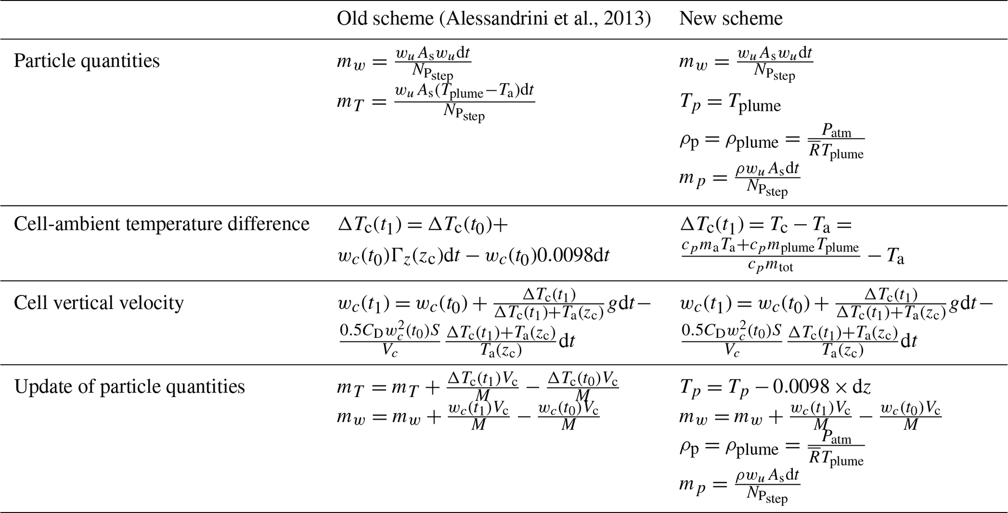
As in the previous algorithm (Alessandrini et al., 2013), the plume rise is calculated using an Eulerian grid. In Alessandrini et al. (2013), at the emission the particles are assigned with an equivalent mass of momentum (m_w) and of temperature difference (m_T) as follows

$$\begin{array}{}\text{(1)}& {\displaystyle }{m}_w={\displaystyle \frac{w_u{A}_{\mathrm{s}}\left|w_u\right|\mathrm{d}t}{N_{{\mathrm{P}}_{\mathrm{step}}}}}\text{(2)}& {\displaystyle }{m}_T={\displaystyle \frac{(T_{\mathrm{plume}}-T_{\mathrm{a}})A_{\mathrm{s}}\left|w_u\right|\mathrm{d}t}{N_{{\mathrm{P}}_{\mathrm{step}}}}}\end{array}$$

where w_u is the plume exit velocity, A_s is the source area, d$t=t_{\mathrm{1}}-t_{\mathrm{0}}$ is the time step, $N_{{\mathrm{P}}_{\mathrm{step}}}$ is the number of particles emitted in the time step, T_plume is the temperature of the emitted plume and T_a is the ambient temperature at the source location. $A_{\mathrm{s}}\left|w_u\right|\mathrm{d}t$ is the volume occupied by the particles in the time step dt.

Afterwards, for the time t₀, the temperature difference between each cell of the Eulerian grid and the environment (ΔT_c), as well as its vertical velocity (w_c), are calculated by summing the contributions of particles contained within the cells themselves

$$\begin{array}{}\text{(3)}& \mathrm{\Delta }{T}_{\mathrm{c}}\left(t_{\mathrm{0}}\right)={\displaystyle \frac{{\sum }_{i=\mathrm{1}}^M{m}_{\mathrm{Ti}}}{V_{\mathrm{c}}}}\end{array}$$

$$\begin{array}{}\text{(4)}& w_c\left(t_{\mathrm{0}}\right)={\displaystyle \frac{{\sum }_{i=\mathrm{1}}^M{m}_{\mathrm{wi}}}{V_{\mathrm{c}}}}\end{array}$$

where M is the number of particles within the cell and V_c is the cell volume.

After the lagrangian advancement of the particles at time t₁, the cell quantities are updated using the following equation for temperature difference

$$\begin{array}{}\text{(5)}& \mathrm{\Delta }{T}_{\mathrm{c}}\left(t_{\mathrm{1}}\right)=\mathrm{\Delta }{T}_{\mathrm{c}}\left(t_{\mathrm{0}}\right)+w_c\left(t_{\mathrm{0}}\right){\mathrm{\Gamma }}_z\left(z_{\mathrm{c}}\right)\mathrm{d}t-w_c\left(t_{\mathrm{0}}\right)\mathrm{0.0098}\mathrm{d}t\end{array}$$

where z_c is the cell height, Γ(z_c) is the lapse rate of the ambient air at cell height z_c and 0.0098 is the adiabatic lapse rate. This temperature difference is used to retrieve the vertical velocity of the cell as follows

$$\begin{array}{}\text{(6)}& \begin{array}{rl}{w}_c\left(t_{\mathrm{1}}\right)& =w_c\left(t_{\mathrm{0}}\right)+{\displaystyle \frac{\mathrm{\Delta }{T}_{\mathrm{c}}\left(t_{\mathrm{1}}\right)}{\mathrm{\Delta }{T}_{\mathrm{c}}\left(t_{\mathrm{1}}\right)+T_{\mathrm{a}}\left(z_{\mathrm{c}}\right)}}g\mathrm{d}t\\ & -{\displaystyle \frac{\mathrm{0.5}{C}_{\mathrm{D}}{w}_c^{\mathrm{2}}\left(t_{\mathrm{0}}\right)S}{V_c}}{\displaystyle \frac{{\mathit{\rho }}_{\mathrm{p}}}{{\mathit{\rho }}_{\mathrm{a}}}}\mathrm{d}t\\ & =w_c\left(t_{\mathrm{0}}\right)+{\displaystyle \frac{\mathrm{\Delta }{T}_{\mathrm{c}}\left(t_{\mathrm{1}}\right)}{\mathrm{\Delta }{T}_{\mathrm{c}}\left(t_{\mathrm{1}}\right)+T_{\mathrm{a}}\left(z_{\mathrm{c}}\right)}}g\mathrm{d}t\\ & -{\displaystyle \frac{\mathrm{0.5}{C}_{\mathrm{D}}{w}_c^{\mathrm{2}}\left(t_{\mathrm{0}}\right)S}{V_c}}{\displaystyle \frac{\mathrm{\Delta }{T}_{\mathrm{c}}\left(t_{\mathrm{1}}\right)+T_{\mathrm{a}}\left(z_{\mathrm{c}}\right)}{T_{\mathrm{a}}\left(z_{\mathrm{c}}\right)}}\mathrm{d}t\end{array}\end{array}$$

where T_a (z_c) is the ambient air temperature at height z_c, g is the gravitational acceleration, S is the cell horizontal cell cross section, C_D is the drag coefficient and ρ_a and ρ_p are the ambient air and plume density, respectively. To move from density to temperature (more easily handled) the ideal gas law was used. In previous works (Tenti and Ferrero, 2024a, b) the dependence of the model on the value chosen for the drag coefficient has been investigated: different formulations dependent on the Reynolds number have been tested, and most tend to asymptotically approach a value of 0.47. Here, we have chosen to use a constant value (C_D=0.5) because calculating this value at each iteration is computationally demanding for the model, and the result tends to approximate a value that is essentially constant anyway.

After the Lagrangian advancement, the temperature difference, and velocity masses of the particles are updated based on the temperature difference and velocity of the cell in which they are located at times t₀ and t₁

$$\begin{array}{}\text{(7)}& \begin{array}{rl}& m_T=m_T+{\displaystyle \frac{\mathrm{\Delta }{T}_{\mathrm{c}}\left(t_{\mathrm{1}}\right)V_{\mathrm{c}}}{M}}-{\displaystyle \frac{\mathrm{\Delta }{T}_{\mathrm{c}}\left(t_{\mathrm{0}}\right)V_{\mathrm{c}}}{M}}\\ & m_w=m_w+{\displaystyle \frac{w_c\left(t_{\mathrm{1}}\right)V_{\mathrm{c}}}{M}}-{\displaystyle \frac{w_c\left(t_{\mathrm{0}}\right)V_{\mathrm{c}}}{M}}\end{array}\end{array}$$

In the new scheme, we want to simulate the transport of heat by assigning to the particles a momentum mass (m_w) as described in Eq. (1), a temperature (T_p), a mass (m_p) and a denisty (ρ_p). The temperature and the density, computed using the ideal gasses law, are those of the plume

$$\begin{array}{}\text{(8)}& {\displaystyle }{T}_p=T_{\mathrm{plume}}\text{(9)}& {\displaystyle }{\mathit{\rho }}_{\mathrm{p}}={\mathit{\rho }}_{\mathrm{plume}}={\displaystyle \frac{P_{\mathrm{atm}}}{\stackrel{\mathrm{‾}}{R}{T}_{\mathrm{plume}}}}\end{array}$$

where P_atm is the atmospheric pressure and $\stackrel{\mathrm{‾}}{R}$ is the gas constant for dry air. The mass is given as

$$\begin{array}{}\text{(10)}& m_p={\displaystyle \frac{\mathit{\rho }{w}_u{A}_{\mathrm{s}}\mathrm{d}t}{N_{{\mathrm{P}}_{\mathrm{step}}}}}\end{array}$$

where w_uA_sdt is the volume occupied by the particles in the first temporal step (dt). Here we are considering the plume as a perfect gas with the same features as the air (same gas specific constant $\stackrel{\mathrm{‾}}{R}$) and specific heat c_p) and we are considering a constant pressure. These assumptions are reasonable approximations since the effects introduced by considering these differences are mostly negligible.

The temperature of the cell (T_c) derives from Richmann's equation for the mixing of two fluids with different temperatures

$$\begin{array}{}\text{(11)}& (c_{\mathrm{1}}{m}_{\mathrm{1}}+c_{\mathrm{2}}{m}_{\mathrm{2}})T_{\mathrm{finale}}=c_{\mathrm{1}}{m}_{\mathrm{1}}{T}_{\mathrm{1}}+c_{\mathrm{2}}{m}_{\mathrm{2}}{T}_{\mathrm{2}}\end{array}$$

where c₁ and c₂ and T₁ and T₂ are the specific heats and the temperatures of the two fluids respectively. As previously mentioned we are considering $c_{\mathrm{1}}=c_{\mathrm{2}}=c_p$ so that Eq. (11) becomes

$$\begin{array}{}\text{(12)}& \begin{array}{rl}{T}_{\mathrm{c}}& ={\displaystyle \frac{c_p{m}_{\mathrm{a}}{T}_{\mathrm{a}}+c_p{m}_{\mathrm{plume}}{T}_{\mathrm{plume}}}{c_p{m}_{\mathrm{tot}}}}\\ & ={\displaystyle \frac{({\mathit{\rho }}_a{V}_c-{\mathrm{\Sigma }}_{i=\mathrm{1}}^M{m}_{\mathrm{pi}})T_{\mathrm{a}}+{\mathrm{\Sigma }}_{i=\mathrm{1}}^M{m}_{\mathrm{pi}}{T}_{\mathrm{pi}}}{{\mathit{\rho }}_{\mathrm{c}}{V}_c}}\end{array}\end{array}$$

where m_a is the mass of the environmental air contained in the cell, m_tot is the total mass contained in the cell considering the air and the plume, $m_{\mathrm{plume}}={\mathrm{\Sigma }}_{i=\mathrm{1}}^M{m}_{\mathrm{pi}}$ is the total mass of the plume contained in the cell, obtained by summing the masses of all the particles within the cell and ρ_c is the cell density. The final density of the cell can be expressed as the total mass (air + plume particles) divided by the total volume (air + plume particles)

$$\begin{array}{}\text{(13)}& {\mathit{\rho }}_{\mathrm{c}}={\displaystyle \frac{m_{\mathrm{a}}+m_p}{V_{\mathrm{a}}+V_{\mathrm{p}}}}={\displaystyle \frac{{\mathit{\rho }}_a{V}_{\mathrm{a}}+{\mathit{\rho }}_p{V}_{\mathrm{p}}}{V_{\mathrm{a}}+V_{\mathrm{p}}}}\end{array}$$

where V_a and V_p are the volumes occupied by the air and the plume particles rispectively.

Once the cell temperature has been computed, we estimate the temperature difference between the cell and the ambient substracting the air temperature

$$\begin{array}{}\text{(14)}& \mathrm{\Delta }T\left(t_{\mathrm{1}}\right)=T_{\mathrm{c}}-T_{\mathrm{a}}\end{array}$$

and this temperature difference is used in Eq. (6) to calculate the vertical velocity.

(Alessandrini et al., 2013)

Table 1 Differences and similarities between old and new scheme.

The vertical velocity of the cell is assigned to the particles inside that cell and it is used to calculate the vertical displacement (dz) of the particles as follows

$$\begin{array}{}\text{(15)}& \mathrm{d}z=w_c\left(t_{\mathrm{1}}\right)\cdot \mathrm{d}t\end{array}$$

According to this new algorithm, the particles move adiabatically, so that their temperature changes only due to the vertical lifting

$$\begin{array}{}\text{(16)}& T_p=T_p-\mathrm{0.0098}\times \mathrm{d}z\end{array}$$

The adiabatic assumption derives from the fact that the characteristic time of the particle displacement is less than the time necessary for a heat exchange between the particles and the ambient to occur.

Table 1 highlights and summarizes the differences between the two schemes.

3 Results

Following the example of Alessandrini et al. (2013), the results obtained with the new plume rise scheme are compared with the Briggs (1975) formula for the plume height for the neutral case

$$\begin{array}{}\text{(17)}& \mathrm{\Delta }h\left(t\right)={\left({\displaystyle \frac{\mathrm{3}}{{\mathrm{0.6}}^{\mathrm{2}}}}{F}_{\mathrm{M}}{\displaystyle \frac{t}{u}}+{\displaystyle \frac{\mathrm{3}}{\mathrm{2}\times {\mathrm{0.6}}^{\mathrm{2}}}}{F}_{\mathrm{B}}{\displaystyle \frac{t^{\mathrm{2}}}{u}}\right)}^{\mathrm{1}/\mathrm{3}}\end{array}$$

where F_M and F_B are the momentum and the buoyancy fluxes respectively, t is the time and u is the ambient wind speed. In order to carry out this comparison, two simulations were performed in an idealized atmosphere, characterized by a constant horizontal wind of 3 and 5 m s⁻¹. The stack height is 120 m and the diameter is 4.5 m. The plume exit velocity is 21.4 m s⁻¹, the plume temperature is 439 K and the ambient air temperature at the stack height is 298 K, with an adiabatic constant vertical temperature profile. In this case the ambient turbulence is horizontally homogeneous and vertically distributed according to Hanna (1982) parametrization.

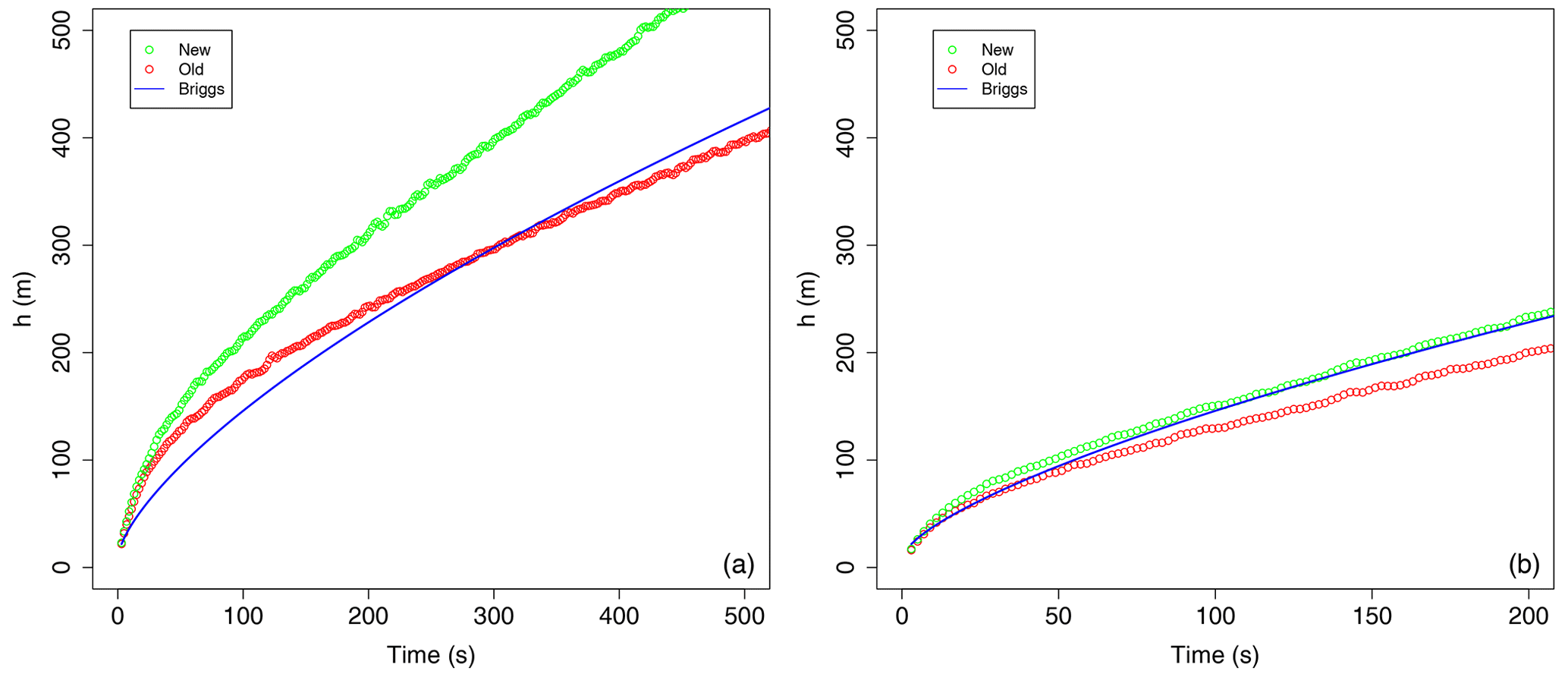
Figure 1 Plume average vertical rise as a function of the time in neutral condition with a constant 3 m s⁻¹ wind speed. (a) Wind speed 3 m s⁻¹, (b) wind speed 5 m s⁻¹. Red circles lines represent simulations with the old scheme (Alessandrini et al., 2013), green circles lines the new scheme, continuous lines Briggs equation (Eq. 17).

To compare the model with experimental data we considered measurements taken during the water tank experiment by Huq and Stewart (1996), in which they replicated a neutral stratified turbulent flow condition and conducted measurements and analysis on the dispersion of a buoyant plume originating from a single point source. Since the experiments are conducted in a water tank, in order to set up a simulation with a Lagrangian model, the scaling factors are calculated based on Froude number similitude and on the assumption $\frac{\mathrm{\Delta }\mathit{\theta }}{\mathit{\theta }}=-\frac{\mathrm{\Delta }\mathit{\rho }}{\mathit{\rho }}$, where ρ is the water density and θ is the potential temperature. The turbulent variables are estimated using the standard deviations of velocities and the dissipation rate of the turbulent kinetic energy. For all our simulations we set the drag coefficient to a constant value (C_D=0.5). In Fig. 1 the results obtained in an idealized atmosphere with a constant wind speed of 3 m s⁻¹ (left) and 5 m s⁻¹ (right) are presented: The red circles' lines are the results of the simulations obtained with the old plume rise scheme (Alessandrini et al., 2013), the green circles lines are the simulations results with the new one, and the continuous blue line is the height obtained with the Briggs equation (Eq. 17).

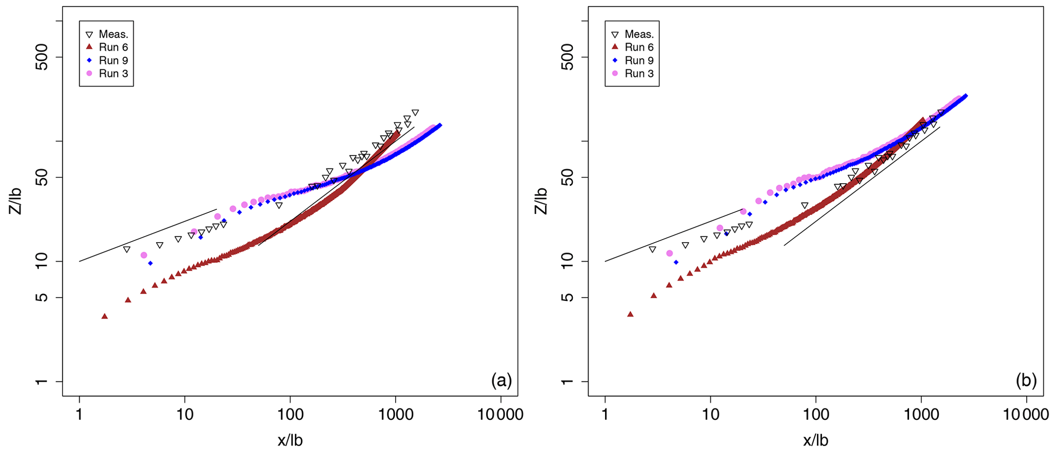
Figure 2 Normalized elevation of the plume centerline as a function of the normalized downwind distance from the source with the old plume rise scheme (a) and the new scheme (c). Triangles indicate the measurements from Huq and Stewart (1996). The coloured symbols refer to the three simulations of the different experiments. The two continuous black lines indicate the $\mathrm{1}/\mathrm{3}$ and $\mathrm{2}/\mathrm{3}$ power-law slopes

In general, with the new scheme, the plume rises more, especially when the wind speed is lower (Fig. 1, left). This could be linked to the fact that we are considering the rise of the particles to be perfectly adiabatic when instead minimal heat exchange occurs. Although the plume with the new algorithm is higher than with the old one, the asymptotic trend is very similar to the Briggs curve. When the wind speed is higher (Fig. 1, right) the height of the particles simulated with the new scheme overlaps perfectly with the Briggs curve (green circles), while with the old scheme (red circles), the plume is slightly lower.

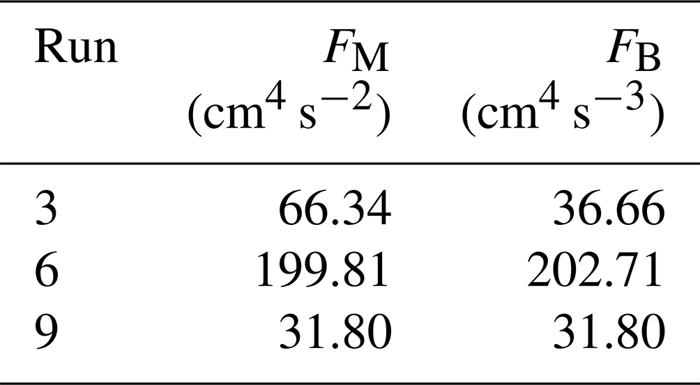
Figure 2 shows the comparison with the experimental data (Huq and Stewart, 1996) with the old scheme (left) and the new scheme (right). The three different runs are characterized by different momentum (F_M) and buoyancy fluxes (F_B) as stated in Table 2.

Table 2 Fluxes of momentum and buoyancy for the 3 different runs

The black lines in the plots represent the trend of the plume height according to the Briggs curve (Eq. 17). Close to the source, the mechanical momentum prevails and the plume should follow the $\mathrm{1}/\mathrm{3}$ power law trend, while moving further away the buoyancy flux begins to prevail and therefore the plume's trend should follow the $\mathrm{2}/\mathrm{3}$ power law trend. In the plots, both the results obtained with the simulations and the measurements are scaled with the buoyancy length scale ($l_{\mathrm{B}}=\frac{F_{\mathrm{B}}}{u^{\mathrm{3}}}$), to be able to compare the results of runs with different characteristics.

As for the near-source field we found similar behaviors with both the schemes, while they differ far from the source, in the $\mathrm{2}/\mathrm{3}$ power-law slope regime. With the old scheme (Fig. 2, left), similar results were obtained for the runs with similar buoyancy flux (3 and 9) and these, although showing a correct asymptotic trend, differ from the experimental measurements. Run 6, having a different value of F_B, tends to align with the measurements. On the other hand, with the new scheme (Fig. 2, right), all runs tend to collapse onto the same values, resulting in better agreement with the measurements.

After comparisons with the Briggs curve and experimental data, the new plume rise scheme gives similar results to the old one but it seems to better reproduce the experimental data.

4 Conclusions

In this study, we introduced a novel plume rise scheme based on heat transport by particles. This method simulates entrainment through the mixing of two fluids – air and plume particles – at different temperatures, with the resultant temperature calculated using Richmann's law. We compared this new algorithm with the existing one in SPRAY-WEB, developed by Alessandrini et al. (2013). Both approaches employ an Eulerian grid to determine plume characteristics, particularly vertical velocity and temperature differential with the external environment. The primary distinction lies in the treatment of particles: while Alessandrini et al.'s (2013) model assigns particles with momentum and temperature difference, our new algorithm also includes mass and density to better simulate heat transport. We evaluated the performance of both algorithms against the analytical Briggs curve in an idealized atmosphere and against experimental data from a water tank experiment. Our findings indicate that the new scheme performs better at higher ambient wind speeds, while maintaining correct asymptotic behavior at lower speeds. Comparisons with experimental measurements reveal that the new algorithm enhances model performance, accurately replicating experimental data regardless of the buoyancy flux involved.