 | 08 Jul 2019
An efficient multi-resolution grid for global models and coupled systems
The latitude-longitude (lat-lon) grid is the most widely used global coordinate system for various purposes but its singularity at the Pole and the vector polar problems associated with its converging meridians hinder its applications. Well from the very start of numerical modelling history, quite a few grids have been attempted to tackle these problems and reduced grid is the simplest one among other grids. However, the reduced grid is almost abandoned by modern numerical modellers due to its unsatisfactory results for dynamical models in the polar region. Spherical multiple-cell (SMC) grid is similar to the reduced grid apparently but uses the unstructured technique for efficiency. It merges longitudinal cells at high latitudes like the reduced grid to overcome the CFL restriction and introduces a polar cell to remove the polar singularity. It also supports quad-tree-like mesh refinement to form a multi-resolution grid. To tackle the vector polar problem associated with the increased curvature at high latitudes, the SMC grid uses a new fixed reference direction to define vector components near the poles for improved polar performance. Global transportation is quite efficient on the SMC grid with optional second or third order transportation scheme. Present applications of the SMC grid, particularly in ocean surface wave models, are presented and possible future usage in global models and coupled systems are proposed.
- Article
(12219 KB) - Full-text XML
- BibTeX
- EndNote


The works published in this journal are distributed under the Creative Commons Attribution 4.0 License. This license does not affect the Crown copyright work, which is re-usable under the Open Government Licence (OGL). The Creative Commons Attribution 4.0 License and the OGL are interoperable and do not conflict with, reduce or limit each other.
© Crown copyright 2019
The latitude-longitude (lat-lon) grid is the most widely used global coordinate system for various purposes and it is used in many operational and research models for its simplicity and convenience. With increased data assimilation in operational models and coupled systems, its convenience becomes even more obvious or indispensable. However, its singularity at the Pole and the vector polar problems associated with its converging meridians have hindered its applications and reduced its efficiency. Well from the very start of numerical modelling history, quite a few grids have been attempted to tackle these problems and reduced grid is the simplest one among other tested grids. But the reduced grid is almost abandoned by modern numerical modellers due to its unsatisfactory results for dynamical models in the polar region (Staniforth and Thuburn, 2012).
The Arctic sea ice coverage has shrunk at alarming speeds in summers of this century. For instance the sea ice edge retreated to as high as the North Pole in the summer of 2016. The disappearing Arctic summer sea ice has led to increased marine activities in the region and hence the demand for research and forecast in the Arctic. The spherical multiple-cell (SMC) grid (Li, 2011) is developed for the Met Office wave forecasting model to cover the newly exposed Arctic sea surface. The SMC grid is a combination of the lat-lon grid and unstructured grid technology. It merges longitudinal cells at high latitudes like the reduced grid (Rasch, 1994) to relax the Courant-Friedrichs-Lewy (CFL) restriction on the Eulerian advection time-step. A polar cell is introduced to remove the singularity at the Pole. As it uses the lat-lon grid quadrilateral cells, numerical modes are minimized and the simple finite-difference schemes on lat-lon grids are retained together with some cell size factors. It also supports quad-tree-like mesh refinement to form a multi-resolution grid (Li, 2012). To tackle the vector polar problem associated with the increased curvature at high latitudes, the SMC grid uses a new fixed reference direction to define vector components near the poles for improved polar performance (Li, 2016).
Global tracer transportation is quite efficient on the SMC grid with optional second or third order transportation scheme, thanks to the removal of the CFL restriction at high latitudes and parallelization of unstructured 1-D arrays. Possible dynamical application on the SMC grid is demonstrated with a model of shallow-water equations (Li, 2018). Its potential applications for global models and coupled systems are to be explored. Starting with a brief outline of the SMC grid technical structure, present applications in ocean surface wave models are demonstrated, followed with some possible future applications in other systems.
A global 6–50 km SMC grid for an ocean surface wave model is shown in Fig. 1. For clarity, only the Euro-Arctic region is shown here. The highest resolution of the SMC grid (size-1) cell is set to be and . So the smallest latitudinal grid length is about 6 km. Because of the unstructured feature of the SMC grid, SMC grid supports flexible domain shapes and stepped resolutions. The SMC wave model grid uses only sea points (or cells) and coastlines are resolved with refined 6 km cells. Away from the coast three times of doubling in cell sizes result in a global 4-level (6–12–25–50 km) SMC grid on ocean surface. So the vast open sea surface is covered with 50 km cells. At high latitudes cells are merged longitudinally following the same rules in Li (2011) to relax the CFL restrictions, ending with eight level 4 cells with Δi=512 and Δj=8 around the polar cell. A unique 4-element integer array is assigned to each cell to hold its SW corner x-, y-indices (i,j), and cell x-, y-sizes (Δi, Δj). The x- and y-indices are measured in size-1 cell increments (Δφ and Δλ) so cell centre latitude and longitude can be worked out with
where λ0 and φ0 are the origin of the cell x- and y-indices. For the SMC 6–50 km grid, the origin of the grid is set at zero-meridian on the Equator so both λ0 and φ0 are zero. The mapping rule Eq. (1) is exactly the same as that for the lat-lon grid cells except for that the SMC grid cells are not arranged in spatial sequence (hence is called an unstructured grid) and their sizes may change by a multiple of 2 (size-1, 2, 4, 8, …). The cells are listed as a 1-D array and sorted by their y-size for use of sub-time steps on refined cells. Please note that the sorting is on the y-size because the cell x-size may change due to the longitudinal merging at high latitudes, which are not counted as resolution level change. The cell number counts in y-size are used for setting up sub-time-step loops for efficient spatial propagation schemes (Li, 2012).
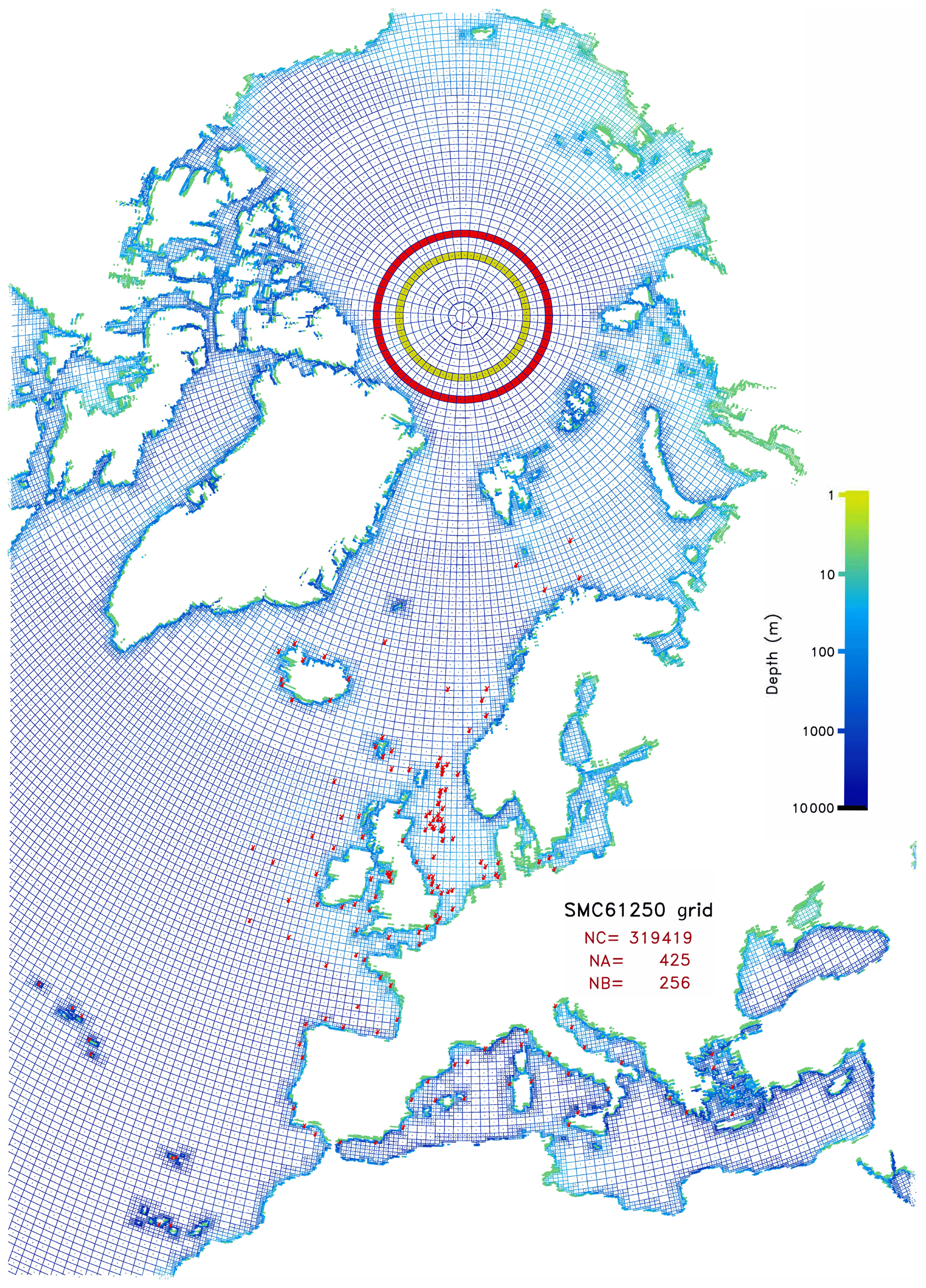
Figure 1The SMC 6–50 km grid.
Because the SMC grid uses the same lat-lon quadrilateral cells as a conventional lat-lon grid, numerical schemes for propagation on the SMC grid are almost identical to those used on a lat-lon grid except for extra size factors for fluxes. The upstream nonoscillatory 2-nd (UNO2) and 3-rd (UNO3) order advection schemes (Li, 2008) have been implemented on the SMC grid. The UNO2 scheme is an improved version of the MINMOD scheme (Roe, 1985) and is the fastest 2-nd order nonoscillatory advection scheme as far as the author knows. The UNO3 scheme is similar to the ULTIMATE scheme (Leonard, 1991) but replaces its flux limiters with the UNO2 scheme. Retaining the lat-lon grid finite difference schemes on the SMC grid is a major advantage over triangle-cell or other shaped finite element grids. It is a well known fact that finite element method is more expensive than finite difference method because of the skewness of finite element cells, which incur more complicated calculation of flow movement than quadrilateral cells. In fact, propagation on this 4-level 6–50 km resolution SMC grid is even faster than that on a conventional 50 km single resolution lat-lon grid because of the relaxed CFL restriction on time step.
In the polar region, SMC grid uses a single Polar cell to remove the singularity at the Pole and introduces a fixed reference direction, the map-east, to mitigate the errors caused by the increased curvature at high latitudes (Li, 2016). The map-east reference direction can be approximated by a rotated grid with its rotated pole at 180∘ E on the Equator. The angle from this approximated map-east to the local east at longitude λ and latitude φ is given by:
Or in the form of rotation coefficients:
Vector components, such as those for wind velocity or 2-D wave energy spectrum, are specified in the map-east direction system at high latitudes (within the red circle in Fig. 1) while the standard local east direction system is used outside the polar region. Because the angle from the map-east to the local east varies with latitude and longitude, vector components defined by local east cannot be mixed up with those defined from the map-east. The map-east region is separate from the local east part and they are linked up by boundary conditions over four overlapping rows. This map-east region is a key feature to improve the polar performance of the reduced grid, particularly for dynamical models (Li, 2018).
Propagation on the SMC grid is calculated in two steps: (1) individual face flux on each cell face is calculated in a face loop based on pre-calculated face information (location, size, and surrounding cells); (2) net flux into each cell is accumulated and used to update cell value in a cell loop. Both the face and cell loops are divided into sub loops by their sizes and sub time steps are used for refined face and cell loops for efficiency (Li, 2012). This sub loop technique makes the multi-resolution SMC grid more efficient than nested grids because of the removal of overlapping regions and boundary conditions in nested systems. The flexible refinement of the unstructured SMC grid makes it even more efficient than conventional nested grids because it does not need to keep a whole rectangular sub-domain at high resolution. For instance, the SMC 6–50 km grid wave model costs less than 2 times of that of a 50 km single resolution SMC grid wave model despite of the refined resolutions and more than doubled cell number.
It has to be emphasized that the map-east polar system is only required for vector components. For propagation of scalars, such as temperature, salinity, atmospheric species or pollutants, there is no need to bother about the curvature at high latitudes as long as the wind components for propagation are given correctly on the SMC cell faces (C-grid). This will be particular useful for a global chemistry model where over a hundred of species may be involved. This scalar transport on a SMC grid is shown in Li (2011) and its computation is much faster than those on the conventional lat-lon grid because of the relaxed time steps and its efficient UNO2 scheme. If an implicit but fast LU decomposition vertical transport scheme is combined with the SMC grid horizontal scheme as in Li (2003) for an air-pollution model, it could build a fast global tracer transportation framework for climate models or Earth systems.
Here a solid body rotation for a scalar field is used to illustrate the SMC grid transport scheme on a full global SMC 1∘ grid as shown in Fig. 2a. It uses a single resolution at and and merged cells at high latitudes. A solid-body rotation angular speed of 10∘ per hour is used and it is equivalent to a full circle of 36 h. The time-step is set to be 120 s so a full cycle takes 1080 time steps. The initial condition is a spherical step function (SSF), which is constructed by setting all cell values to be 1.0 unit except for cells within a 20∘ wide stripe along the Equator. Cells within this stripe are initially set to be 5 units (as marked by the red dots in Fig. 2a). The initial SSF is shown in Fig. 2b and its maximum value 5.0 and minimum value 1.0 are printed in the lower-left corner. The rotational pole is chosen on the Equator so the raised stripe ring could sweep over the full sphere. The SSF sharp ring edges are very sensitive to numerical oscillations and the uniform background is ideal to reveal any distortion caused by the advection scheme or the size-changing parallels.
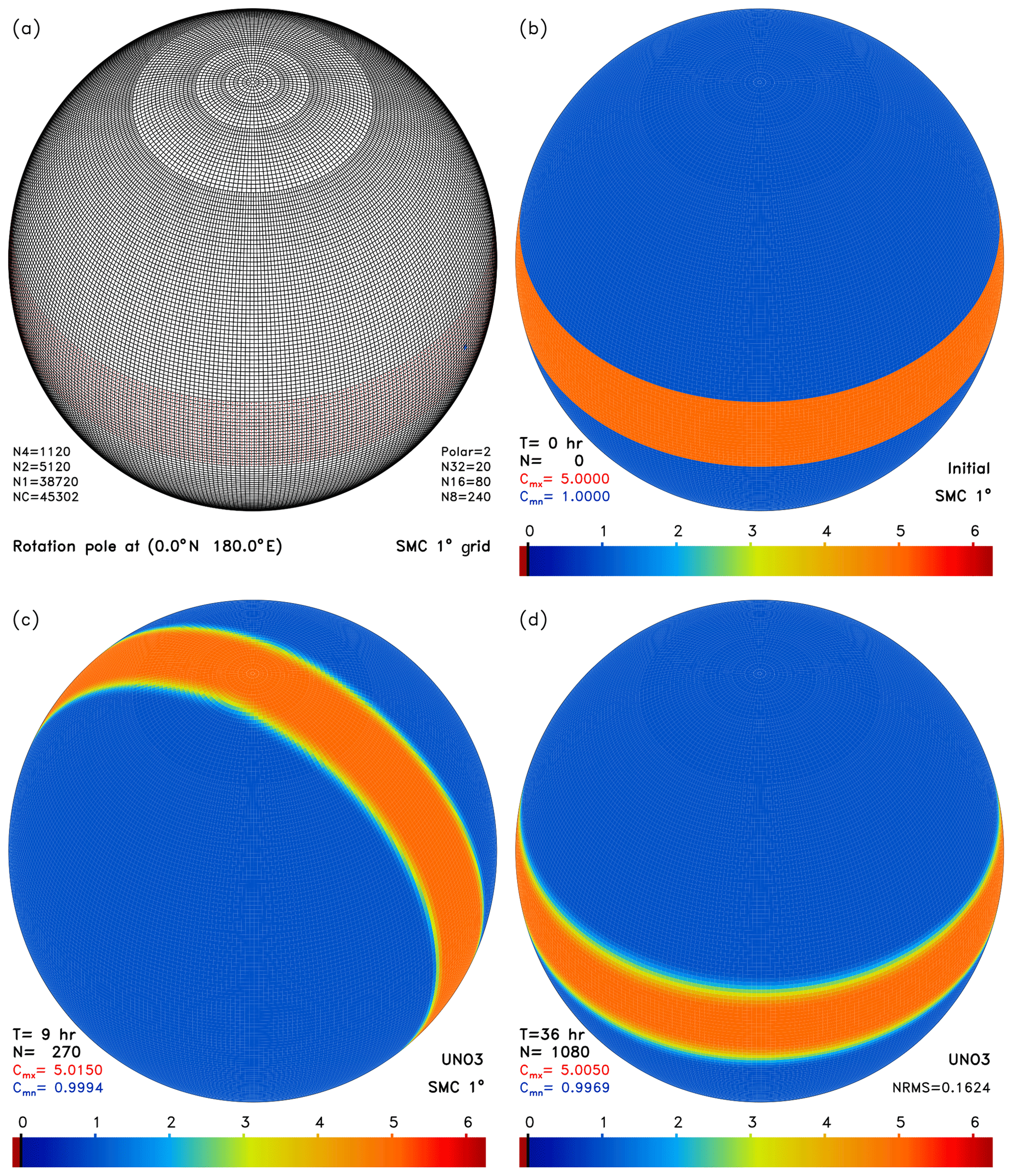
Figure 2c shows the simulated result with the UNO3 scheme after 90∘ rotation when the raised stripe is just over the Poles. The maximum and minimum values are 5.015 and 0.9994 units, respectively, indicating some small oscillations near the stripe edges. Nevertheless, the whole background and the raised stripe look unchanged except for the rounded stripe edges. This indicates that the SSF passes through the size-changing parallels and the polar cells smoothly. Fig. 2d shows the solid-body rotation result after one full cycle at t=36 h. The maximum and minimum values (5.005 and 0.9969) indicate that the small oscillation at the stripe edges persists but is smaller than when the stripe crosses the Pole (Fig. 2c). By this time, the stripe has returned back to its initial position so a normalised root-mean-square (NRMS) error could be evaluated against the initial SSF. The SSF one-cycle NRMS error on the SMC 1∘ grid with the UNO3 scheme is 0.1624. Using the UNO2 scheme on the SMC 1∘ grid for rotation of the same SSF shows a very similar result except for a slightly enhanced smoothing. The SSF one-cycle NRMS error for UNO2 is 0.2161 with the same angular speed and time step as in the UNO3 test.
Physical diffusion or numerical smoothing may degrade high order advection scheme and makes it equivalent to a low order scheme. For instance the UNO3 scheme plus a diffusion term yields similar results as that of the UNO2 scheme (Li, 2008). Considering the UNO2 scheme is about 30 % faster than UNO3, the small loss of accuracy by UNO2 is worthwhile, especially if smoothing is required or physical diffusion is present as in the atmosphere. The SMC grid has been implemented into an ocean surface wave model (WAVEWATCH III Development Group, 2016) and has been validated with observations (Li, 2012). The map-east system has been tested in an idealised ice-free Arctic and validated with available satellite observations (Li, 2016). Although both UNO2 and UNO3 are available for the SMC grid in the WAVEWATCH III wave model, they produce almost identical ocean surface wave field because a strong numerical smoothing is used to control the so called garden sprinkler effect in the wave spectral field (Li, 2012). So the UNO2 advection scheme and the SMC grid combination is strongly recommended for atmospheric dispersion or chemistry model where physical diffusion is unavoidable.
A unified global and regional multi-resolution SMC grid (3–6–12–25 km) wave model has been running for the Met Office operational wave forecast since October 2016 (Li and Saulter, 2014). There is also a regional SMC 3–6–12–25 km grid ensemble wave forecast model running in the Met Office (Bunney and Saulter, 2015). A global SMC 50 km wave model is used in the Met Office coupled system, which allows the wave climate scenario of ice-free Arctic to be simulated. The SMC 6–50 km grid as shown in Fig. 1 is recommended for future update of the wave model component in the Met Office coupled system. A rotated 1.5–3 km SMC grid UK regional wave model is now in preparation to replace the present 4 km rotated lat-lon grid operational wave model in the Met Office. Casas-Prat et al. (2018) used a 50–100 km global SMC grid wave model for their wave climate study, including the entire Arctic Ocean. SMC grid application in dynamical model has not been fully explored yet. Li (2018) discretized shallow-water equations on a full global multi-resolution SMC grid and conducted a few classical tests. Results demonstrated that the two reference directions work well on the SMC grid to suppress numerical errors associated with the vector polar problem. The multi-resolution grid is fine for smooth flow but may stir up instability ripples in strong jet flow. Future study in 3-D dynamical model application is needed.
Spherical multiple-cell (SMC) grid is similar to the reduced grid apparently but is an unstructured grid in nature. It merges longitudinal cells at high latitudes like the reduced grid to overcome the CFL restriction and introduces a polar cell to remove the polar singularity. It also supports quad-tree-like mesh refinement to form a multi-resolution grid with flexible domain shape. It has been used in ocean surface wave models to resolve coastline details with refined cells while keeping the vast open ocean surface at affordable coarse resolution. To tackle the vector polar problem associated with the increased curvature at high latitudes, the SMC grid uses a new fixed reference direction to define vector components near the poles for improved polar performance. This has been used to extend ocean surface wave model at high latitudes to cover the newly exposed sea surface area due to the retreating Arctic summer sea ice. It is also used for wave climate studies to simulate the ice-free Arctic wave environment. Global transportation on the SMC grid is quite efficient with optional second or third order transportation scheme and it is recommended for other global models or Earth systems, particular for scalar tracer transport. Application in dynamical models has been attempted with a model of shallow water equations and further studies are required before it could be implemented into a 3-D model. An even optimal future view is to use a single SMC grid for all the component models in an Earth system or coupled model so it has unique 1-1 grid cell correspondence for exchange of information between different component models. This may greatly simplify the structure of Earth systems or coupled models.
THE SMC grid source code is available from the WAVEWATCH III model public web page: https://github.com/NOAA-EMC/WW3/releases/tag/6.07 (WAVEWATCH III Development Group, 2019). Other queries may be sent to the author by emails.
The author declares that there is no conflict of interest.
This article is part of the special issue “18th EMS Annual Meeting: European Conference for Applied Meteorology and Climatology 2018”. It is a result of the EMS Annual Meeting: European Conference for Applied Meteorology and Climatology 2018, Budapest, Hungary, 3–7 September 2018.
The author is grateful to the editor, Daniel Reinert, and two anonymous referees for their useful comments to improve this article.
This research has been supported by the UK public weather service in the Met Office.
This paper was edited by Daniel Reinert and reviewed by two anonymous referees.
Bunney, C. and Saulter, A.: An ensemble forecast system for prediction of Atlantic-UK wind waves, Ocean Model., 96, 103–116, 2015.
Casas-Prat, M., Wang, X. L., and Swart, N.: CMIP5-based global wave climate projections including the entire Arctic, Ocean Model., 123, 66–85, 2018.
Leonard, B. P.: The ULTIMATE conservative difference scheme applied to unsteady one-dimensional advection, Computer Methods Appl. Mech. Eng., 88, 17–74, 1991.
Li, J. G.: A multiple-cell flat-level model for atmospheric tracer dispersion over complex terrain, Bound.-Lay. Meteorol., 107, 289–322, 2003.
Li, J. G.: Upstream nonoscillatory advection schemes, Mon. Weather Rev., 136, 4709–4729, 2008.
Li, J. G.: Global transport on a spherical multiple-cell grid, Mon. Weather Rev., 139, 1536–1555, 2011.
Li, J. G.: Propagation of ocean surface waves on a spherical multiple-cell grid, J. Comput. Phys., 231, 8262–8277, 2012.
Li, J. G.: Ocean surface waves in an ice-free Arctic Ocean, Ocean Dynam., 66, 989–1004, 2016.
Li, J. G.: Shallow-water equations on a spherical multiple-cell grid, Q. J. Roy. Meteor. Soc., 144, 1–12, 2018.
Li, J. G. and Saulter, A.: Unified global and regional wave model on a multi-resolution grid, Ocean Dynam., 64, 1657–1670, 2014.
Rasch, P. J.: Conservative shape-preserving two-dimensional transport on a spherical reduced grid, Mon. Weather Rev., 122, 1337–1350, 1994.
Roe, P. L.: Some contributions to the modelling of discoutinuous flows, Lectures in Appl. Math., 22, 163–193, 1985.
Staniforth, A. and Thuburn, J.: Horizontal grids for global weather and climate prediction models: a review, Q. J. Roy. Meteor. Soc., 138, 1–26, 2012.
WAVEWATCH III Development Group: User manual and system documentation of WAVEWATCH III version 5.16. Tech. Note 329, NOAA/NWS/NCEP/MMAB, College Park, MD, USA, 326 pp. + Appendices, 2016.
WAVEWATCH III Development Group: Public release version 6.07, available at: https://github.com/NOAA-EMC/WW3/releases/tag/6.07, last access: 1 July 2019.