TITAN automatic spatial quality control of meteorological in-situ observations

In science, poor quality input data will invariably lead to faulty conclusions, as in the spirit of the saying “garbage in, garbage out”. Atmospheric sciences make no exception and correct data is crucial to obtain a useful representation of the real world in meteorological, climatological and hydrological applications. Titan is a computer program for the automatic quality control of meteorological data that has been designed to serve real-time operational applications that process massive amounts of observations measured by networks of automatic weather stations. The need to quality control third-party data, such as citizen observations, within a station network that is constantly changing was an important motivation that led to the development of Titan. The quality control strategy adopted is a sequence of tests, where several of them utilize the expected spatial consistency between nearby observations. The spatial continuity can also be evaluated against independent data sources, such as numerical model output and remote sensing measurements. Examples of applications of Titan for the quality control of near-surface hourly temperature and precipitation over Scandinavia are presented. In the case of temperature, this specific application has been integrated into the operational production chain of automatic weather forecasts at the Norwegian Meteorological Institute (MET Norway). Titan is an open source project and it is made freely available for public download. One of the objectives of the Titan project is to establish a community working on common tools for automatic quality control, and the Titan program represents a first step in that direction for MET Norway. Further developments are necessary to achieve a solution that satisfies more users, for this reason we are currently working on transforming Titan into a more flexible library of functions.

1 Motivations

Applications in meteorology, hydrology and climatology are based on different assumptions, serve different needs and have different objectives. Nevertheless, they all share the fundamental working hypothesis that observed data are representative of the atmospheric state. Unfortunately, this is not always the case, for example with malfunctioning measurement devices. As a consequence, data quality control is needed in every data processing application.

For meteorological observations the same data is used to represent phenomena over a large spectrum of spatial and temporal scales. Therefore, the characterization of the uncertainties of meteorological observations depends on the application at hand, and it might happen that the uncertainty of a particular observation is too large for a specific purpose, even when the observation itself is an accurate measurement of the atmospheric state. As an example, consider a network of automatic weather stations measuring temperature and suppose we want to use it for spatial analysis over a regular grid. A perfect measurement coming from an isolated station located in a “cold pool” surrounded only by distant stations measuring warmer air might introduce inaccurate features in the predicted temperature field: the size of the cold pool could be overestimated, for instance. For some applications, when the estimated uncertainty of an observation is too high, one may decide to exclude that observation.

In the past, and particularly for climatological applications, the data quality assurance system within national meteorological services strongly relied on specialized staff to check the measured data (WMO, 2018). However, having a trained meteorologist or climatologist checking each and every observation by eye is simply impossible due to the exponential increase in the number of available observations, both from the point of view of station locations and sampling frequency. In recent years, a number of non-conventional observations (e.g. citizen science data (Chapman et al., 2017; De Vos et al., 2017, 2019a; Nipen et al., 2019), and measurement from moving vehicles (Anderson et al., 2012, 2019)) have been stored in the databases of national centres alongside conventional observations. Such observations should be treated carefully on their own (Bell et al., 2015), but are valuable because the immense amount of data points leads to a redundancy of neighbours to validate the measurements.

Automatic data quality control procedures are needed to support human-based quality control. In fact, one of the aims of the automatic procedures is to reduce the set of observed data that must be evaluated by experts. For instance, extremes and rare events in general are critically important data because of their impact on human activities and the specialized staff working at national meteorological institutes can then focus on evaluating this data without getting lost in the massive stream of data stored every day (or even every few seconds) in the databases.

Different quality control approaches with focus on timeseries analysis of meteorological data have been proposed and tested on data from citizen networks. Meier et al. (2017) uses four levels of filtering based on checking metadata, and the analysis of the temperature timeseries of citizen stations with reference to a trusted coarser network of stations measuring temperature and radiation. Napoly et al. (2018) uses seven levels of quality control for temperature measurements from citizen stations. The main part checks the metadata, corrects for elevation differences between stations, performs a modified z-score test, and calculates the Pearson correlation coefficient (against the monthly median). The optional part includes interpolation of single missing values and checks for the percentage of data availability per day and per month. De Vos et al. (2019b) uses a default bias correction and checks precipitation measurements for faulty zeroes, high influx, and station outliers (by timeseries comparison) against the median of neighbouring stations within 10 km.

We present (the first version of) the automatic data quality control tool, Titan (https://github.com/metno/titan, 14 July 2020), which is specifically designed to process massive amounts of meteorological data. Titan puts emphasis on spatial controls of the in-situ observations, i.e. we exploit expected spatial consistency and continuity of meteorological fields to detect suspect observations.

The Titan software is open source, written in R (R Core Team, 2015), and developed at the Norwegian meteorological institute (MET Norway).

Titan can be tailored to fit the specific application at hand (e.g. the creation of a climatological gridded dataset or the validation of a dynamic network of citizen observations). The software has the flexibility to handle input from multiple sources and allows the user to specify the level of trust for each source. In this way, networks of different characteristics can be combined. Titan gives a clear answer regarding good/bad observations which is ideal for use in operational chains. The current version is being used operationally at MET Norway for temperature, and is under development for precipitation measurements. We envision applying Titan to other measurements, such as snow depth, relative humidity and atmospheric pressure. It is worth remarking here that the integration of Titan with the human-based quality control at MET Norway is still under development. MET Norway's publicly available observed data, such as the archive accessible via the Frost API at https://frost.met.no/index.html (14 July 2020), are not validated using Titan.

This paper begins by shortly defining the relevant measurement errors that quality control routines should detect. Then, we present the tests of Titan, before giving a few examples of Titan in action. We close with a discussion on planned developments.

1.1 Definitions of errors

Often in atmospheric science we face a problem that can be formulated as follows. We are working on an application that estimates the true value for a variable of interest. As an example, consider the application of monitoring the climate over a region, then we implicitly assume that one of our variables of interest is the spatially aggregated maximum monthly temperature over that region. Observations of this variable are obtained by aggregation of measurements. These are our best estimates of the true values, and include uncertainties quantified by errors.

We follow the error definitions from Gandin (1988). The inherent random errors do not depend on measured values (they are distributed more or less symmetrically around zero), and encompasses both observational errors and representativeness errors. Systematic errors result in biases (i.e. they are distributed asymmetrically around zero), and can come from a scale shift of the instrument or from some persistent factor that is not accounted for. Lastly, there are rough errors, that are large errors from e.g. faulty sensors or from data handling. Gross errors are defined as very large rough errors.

Titan makes available to the user several tests aiming at detecting those observations that are most likely affected by: rough/gross errors, large systematic errors, and especially, large representativeness errors. These are errors that are highly likely to occur in networks that also include citizen observations. If compared to professional stations managed by weather services, citizen observations are suspected of being less reliable due to a lack of metadata, poor placement (e.g. insufficient radiation shielding or proximity to buildings) or possibly non-existing maintenance. Hence, the precautionary principle is assumed, even though our experience shows that the overwhelming majority of citizen observations are representative of the actual atmospheric state (Nipen et al., 2019).

2 Methods

Titan tests the observations from all stations referring to the same observation time simultaneously. This approach is crucial for an observation network that is constantly changing in size. Titan will test each observation with respect to the current available neighbours timestep by timestep, and thus, can handle amateur stations going in and out of the network, and any future inclusion of completely new sources of data.

The Titan code is built up as a series of sequential checks (see Table 1), that require command-line arguments to be triggered. The appropriate compilation of these depends on the application and the meteorological variables at hand. The observations are marked as good if they pass all tests. If an observation fails a test, that one will be marked as bad, and it will not go up against the remaining tests. Afterwards, it is then possible to retrieve information about which test that was failed for each observation.

Table 1 List of sequential checks for temperature and precipitation.

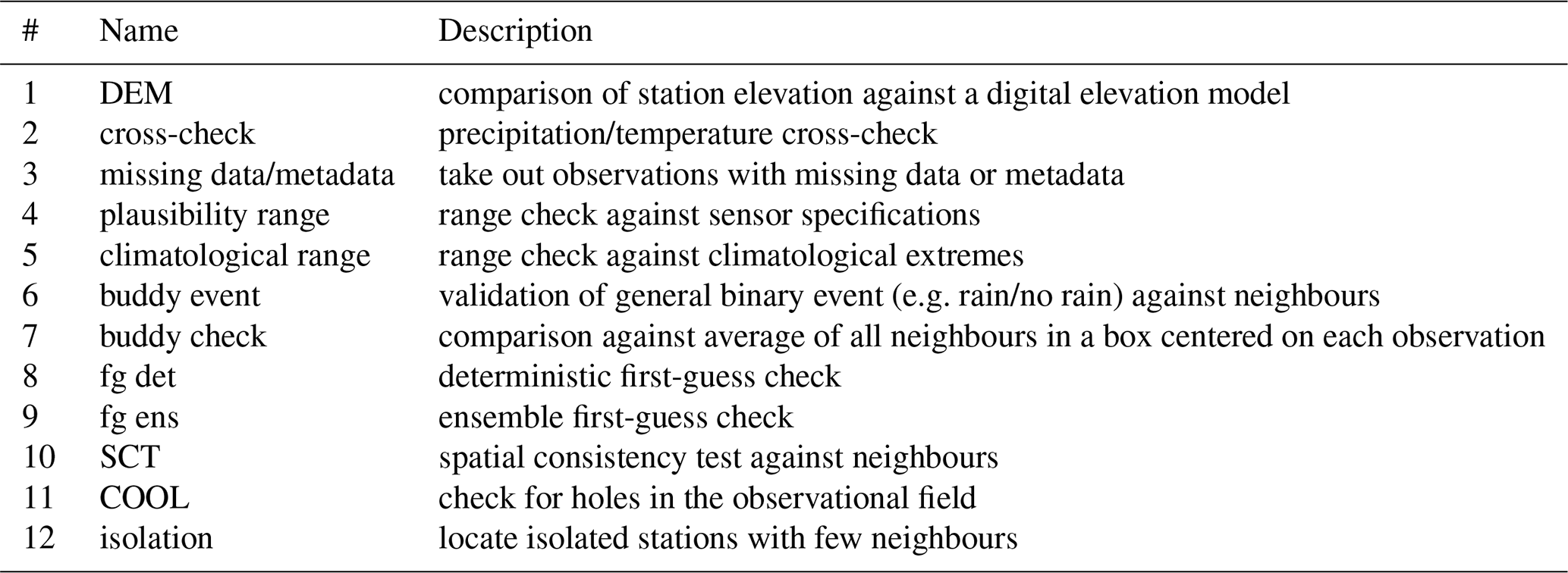
2.1 Tests

The first check is a check of the elevation of the stations providing the observed values against a digital elevation model (e.g. GMTED2010). Observations are flagged as suspicious if the difference between the two is higher than a chosen threshold.

A cross-check between different atmospheric quantities is implemented specifically for precipitation. As discussed by Førland et al. (1996) and Wolff et al. (2015), rain gauges may underestimate precipitation due to undercatch in windy conditions and the underestimation is particularly significant for solid precipitation. In addition, build up of snow might overflow the gauge, or precipitation can be registered at the wrong time when collected snow melts. For these reasons, in-situ precipitation observations can be tested against temperature (extracted from a gridded dataset, e.g. from model), so that one can remove observations from non-heated rain-gauges during winter for negative temperatures.

Next, we have checks for missing data or missing metadata.

These are followed by a plausibility check that is a range check tuned so as to identify implausible observations according to the specification of the sensor's manufacturer.

The observations can also be checked in relation to climatological values. These are observations that can be within the range of plausible values, but outside the range of values typical for the season or particular month in question. As default, we define the climatological thresholds on a monthly basis. The climatological and plausibility checks are both range checks, however, it can be useful to distinguish between the two tests as they return different information that might trigger specific actions. A suspect observation identified by the plausibility check is affected by gross-measurement error, while an observation failing the climatological check may be an extreme.

Then we have two types of “buddy checks”. An event-based buddy check can be applied to dichotomous (or binary) events of the type “yes, the event has happened” or “no, the event has not happened”. In this case, the test is based on the categorical statistics. An event-based buddy check serves the purpose of validating a general event (e.g. rain/no rain) at a station against its neighbours. This test uses the same square-boxes to define the neighbors as is described in detail for the traditional buddy check in the next paragraph, but the test consists of two thresholds. First, there is a limit for creating the binary events to be checked for all observations (this could be above/below 0.1 mm for our rain/no rain example). Then, there is the threshold for accepting or rejecting each of the observations, which is a limit for the conditional probability that a binary event is likely based on the neighbouring stations in the box. This threshold can be set so that an observation is flagged as “suspicious” if the vast majority (e.g. 90 %) of its neighbours measure the opposite category.

A traditional buddy check compares the observations against the average of all neighbours in a square box centered on each observation. The user chooses the distance from the central observation to the sides of the box. A minimum number of observations is required to be available in the box, and the range of elevations must not exceed a specified threshold. One can perform several buddy checks in a row by specifying the desired number of iterations. Any observations flagged as poor quality do not enter the next round. It is also possible to assign priorities to different station providers, so that in the first round of the buddy check, high priority observations are not compared against lower priority observations. Both the use of priorities and the iterative procedure are strategies to avoid flagging good observations that happen to be close to bad ones. In the case of temperature, elevation differences are taken into account by transforming all observations to the elevation of the observation in the center of the box (i.e. the location of the observation undergoing the test) before averaging. This is done by assuming a linear vertical profile of temperature with a lapse rate of −0.0065 ^∘C m⁻¹ as defined in the ICAO international standard atmosphere. In the case of precipitation, the observed values are transformed with a Box–Cox transformation (with a parameter value of 0.5 as default (Erdin et al., 2012)) before undergoing the test, to reduce the risk of erroneously removing small-scale intense precipitation. For the buddy check of both temperature and precipitation, the observation is flagged as suspicious if the deviation between the observed value and the box-average normalized by the box standard deviation exceeds a predefined threshold. The observation under test is excluded from the box statistics. As a general rule, the buddy check aims at identifying outliers, which in climatology are defined as values more than 5 standard deviations from the mean (Lanzante, 1996).

The next option is a deterministic first-guess check that compares in-situ observations against a gridded field (e.g. radar output or the output of a numerical weather prediction model). The test will then flag dry observations while the first-guess field contains precipitation, and vice versa.

An ensemble first-guess version compares the observations against an ensemble of gridded fields (usually the output of a stochastic numerical model). First-guess values at the station locations are extracted by means of bilinear interpolation, and the ensemble members are used to derive the ensemble statistics (mean, standard deviation, quartiles and interquartile range). The observations are checked against the ensemble mean (with a threshold related to standard deviation), and against both ensemble quartiles (with a threshold related to inter-quartile range). There is also a factor to account for underdispersion by the ensemble. Temperature observations are adjusted for elevation differences between the station elevation and the digital elevation model. In case of precipitation, a Box–Cox transformation is applied to both the ensemble values and to the in-situ observed values.

The next test is the spatial consistency test (SCT) which acts as a more sophisticated buddy check by evaluating the likelihood of an observation given the values observed by the neighboring stations. Since the SCT is computationally more expensive than the buddy check, the buddy check is used for thinning the observation dataset before applying the SCT. We refer the reader to Lussana et al. (2010) for an in-depth description of the SCT. It is worth remarking here that the SCT automatically adapts to the local observation density, such that the check is stricter for data dense regions and more flexible for data sparse regions, where the lack of redundancy results in larger uncertainties.

The SCT is performed independently over several sub-domains of a region. The sub-domains can be set up in two ways. One version uses square boxes centred on each observation, as is done for the buddy check. The other version uses a fixed regular grid, that covers the region with observations, and checks each observation against the other observations belonging to the same box. The first will be most accurate as each box contains all the closest neighbours, while the second will be faster and hence benefit operational applications.

The SCT is based on optimal interpolation (OI, Gandin and Hardin, 1965), in the formulation given by Uboldi et al. (2008). Let us consider the case of temperature and the square box centered on the observation to test. A vertical profile is fitted through the temperature observations against elevation of each station within the box, following Frei (2014). This reference profile provides a prior temperature estimate that can be seen as a background or large scale temperature signal. The temperature estimate is obtained without using the observed value at that location. Then, OI is used at the station location to locally adapt the background towards the surrounding observations. OI returns three quantities evaluated at the station location: (1) an independent temperature prediction for the observation under test; (2) the error variance of the predicted value; (3) the error variance of the observed value. These error variances quantify the expected deviation between either the predicted or observed value and the unknown true value. The SCT compares the squared deviation between observed and predicted values, normalized by the sum of their error variances, with a predefined threshold. The observation is flagged as suspicious if the normalized deviation is larger than expected. In this sense, the SCT is similar to the buddy check. It is not possible to define SCT thresholds that are universally valid. The optimal values depend on the specific application and they can be set by considering statistics both over a few years and over some significant case studies. The ideal case would be to tune the thresholds through the comparison of the flagged observations against the outcomes of reliable quality control results, such as those derived from experienced staff checking a subset of the observations.

In the case of temperature, the strong relationship with elevation allows us to express the background in terms of a geographical quantity. A similar situation occurs for atmospheric pressure, for example. When it is not possible to express the background as a function of the geographical parameters, it is advised to use a first guess from numerical models or remote sensing as the background. For instance, in the case of hourly precipitation it is possible to use the output of a numerical model or radar-derived precipitation fields as the first-guesses for the background.

For the SCT and the buddy check, it is possible to specify different thresholds for different providers and for negative and positive deviations of the observed values from the reference values. In this way one can use prior knowledge of expected quality to weight the trust in various data sources. As stated in Sect. 1.1, citizen observations are for example more likely to have poorer quality, and should have stricter thresholds compared to WMO compliant stations. Many citizen stations experience a warm bias due to direct sunlight and proximity to buildings, which in turn allows for stricter thresholds for positive temperatures from these stations.

Note that the first guess checks can be used independently from the SCT or they can be used in support of the SCT. In this last case, the SCT and one of the first-guess checks may be based on the same gridded field. The first-guess checks are then used as a pre-processing step to reduce the number of observations checked by the SCT, which is more computationally expensive.

Then, we have the “check for holes in the field” (COOL) test, which can be particularly useful for precipitation. It detects observations that are responsible for introducing strange patterns such as e.g. dry holes in an area of large scale precipitation. All observations are transformed into binary events given a numerical threshold as for the event-based buddy check. Then, each gridpoint of a finer grid is assigned yes/no based on a nearest neighbor interpolation, giving a gridded field that will be alternating between patches of connected yes/no cells. If a patch of connected cells includes less than a predetermined number of observations, those observations are flagged as suspicious. Observations flagged by the COOL test are not necessarily affected by gross errors, rather there could be too few to properly represent the small-scale process they are observing, where “small-scale” is defined with respect to the local observation density.

Low-quality stations also undergo an isolation test to ensure that there are enough nearby independent sources of information to confirm the measurements. In the current version of Titan, isolated stations are flagged as the last step of the quality control such that the final decision on whether to use them is left to the user.

3 Examples of applications

In the paper by Nipen et al. (2019) the production chain designed to provide automatic weather forecasts of temperature on https://www.yr.no/ (14 July 2020), a popular website for weather forecasts, is described. As a first example of application, in Sect. 3.1 we are describing the Titan setup used for the real-time quality control of the in-situ observational dataset of hourly temperature used in that paper. The dataset includes both professional weather stations, managed by public institutions, and amateur stations owned by private citizens. In Sect. 3.2, a second example of application is presented for the real-time quality control of hourly precipitation and the Titan setup is described. The observational network considered is the same as in the first example, except that in this case we apply Titan to the observations of precipitation and the number of amateur stations equipped with gauges are less than those measuring temperature. It is worth remarking once more that Titan is not used operationally for the quality control of precipitation. Hence, the application of Titan to precipitation data is at a less mature stage of development compared to its application to temperature.

The domain considered in both examples is shown in Fig. 1. It covers Fennoscandia, which is a region characterized by complex terrain, with large inland water bodies, narrow valleys and wide mountainous areas, plus an intricate coastline. The whole network of automatic weather stations to quality control is a composition of several sub-networks managed by different institutions or private companies, each of them having very different interests. The data are divided into three categories, summarizing our prior knowledge (i.e., before any measurement has been taken) of the data quality. In the first category (category I) we find the stations installed and operated by public institutions and that meet the WMO standards (WMO, 2018). In the second category (category II) there are the stations operated by public institutions that do not meet WMO standards. In the third category (category III) there are the stations that have been installed and that are operated in such a way that MET Norway does not have any control on them. Data from stations in the first two categories represents the classical source of in-situ observations used in atmospheric science. The third category includes third-party data, such as amateur weather data, that can be used thanks to their massive redundancy that allows for a reliable spatial quality control. MET Norway gets thousands of citizen observations in Scandinavia thanks to the private company Netatmo, which ensures a steady data stream at a sampling rate of less than 1 h.

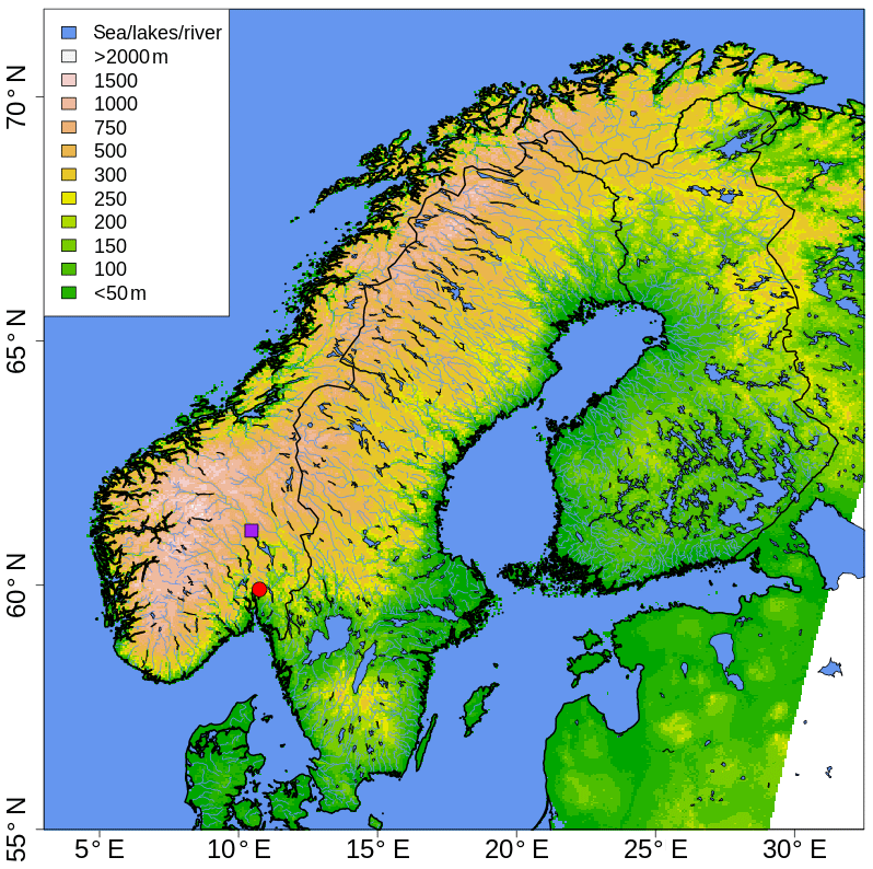
Figure 1 Spatial domain, in the geographical coordinate system, used for the example application. The sea, large bodies of water and rivers are shown in blue. The altitude above the mean sea level (in m) is shown through shaded colors. The red circle marks Oslo. The purple square marks Lillehammer.

For all examples presented in Sect. 3.1 and 3.2, the first check is related to the metadata completeness. Then, the station elevation is compared against the GMTED2010 digital elevation model. Those station locations that deviate from the digital elevation model with more than 500 m are not used with their own elevation but with an elevation extracted from GMTED2010.

3.1 Quality control of hourly temperature

The plausibility check uses the preset thresholds of −50 and 40 ^∘C. We are not using any climatological checks.

Two iterations of the buddy check are performed over all observations without any provider priority. The size of the square box surrounding each observation used to compute the buddy check statistics is 3 km. The square box must contain at least four observations, plus the observation undergoing the test that lies at the center of the box. Observations that are more than two standard deviations from the corresponding expected value are flagged as suspicious. Note that in this case we are implementing a more restrictive test for outliers than what is described in Sect. 2.1. The threshold of two standard deviations has been set after trial and error experiments.

Two SCT-iterations are performed. Since we are testing tens of thousands of observations each hour, we have opted for the fixed-grid setting of the SCT. The domain in Fig. 1 is divided into sub-domains of approximately 100 km × 100 km, then the background field is estimated independently within each sub-domain given the observations in it. Sub-domains that include less than 50 observations are not used for the SCT, because with such a small number of observations the results are not robust enough. In the OI setup we distinguish between stations in the three different categories introduced above. Stations in category I are assumed to be five times more reliable than the background, stations in category II are three times more reliable than the background, while stations in category III are two times more reliable than the background. With respect to the notation used by Uboldi et al. (2008) and Lussana et al. (2019), this corresponds to setting the ratio between the observation and the background error variances to ε²=0.2 (category I), ε²=0.33 (category II) and ε²=0.5 (category III). The OI procedure requires the specification of two reference length scales determining the decrease of influence of one observation over the others with an increase of the distance, in the horizontal and in the vertical directions. The vertical reference length scale is set to 200 m. The horizontal reference length scale is estimated adaptively for each sub-domain as the 10th percentile of the distribution of distances between pairs of stations. This way we ensure that the OI can adjust the large-scale background towards the observed value over wide portions of the sub-domains. The lower bound of the horizontal reference length scale is set to 1 km. The SCT thresholds are also dependent on the observation category. Category I observations are suspicious if they deviate from the corresponding predicted value by more than 12 times the estimated error variance. This threshold reflects our high degree of belief in the quality of these stations. Category II and III observations are suspicious if their deviations exceed four times the error variances for positive temperatures and 8 times the error variances for negative temperatures.

The isolation test is performed after the other tests. Observations not in category I with less than 5 neighbouring stations within a 15 km radius and 200 m elevation difference are flagged as isolated.

We briefly present two cases showing the output of the quality control by Titan using the tests and settings as described above. Figure 2 shows the temperature and SCT score values for 06:00 UTC on 5 November 2019 for the area surrounding Lillehammer, a small city located in a valley in Innlandet county in Norway. The station coverage is sparse, with most observations located close to the valley floor around 125 m a.m.s.l., and some observations along the side of the valley reaching about 500 m a.m.s.l. The temperature is in general around −10 ^∘C for this wintertime morning. None of the observations are way off, but the SCT has in this case flagged a few as suspicious. The SCT scores range from 4.0 (almost accepted) to 12 for the observation close to 61.1^∘ N 10.47^∘ E.

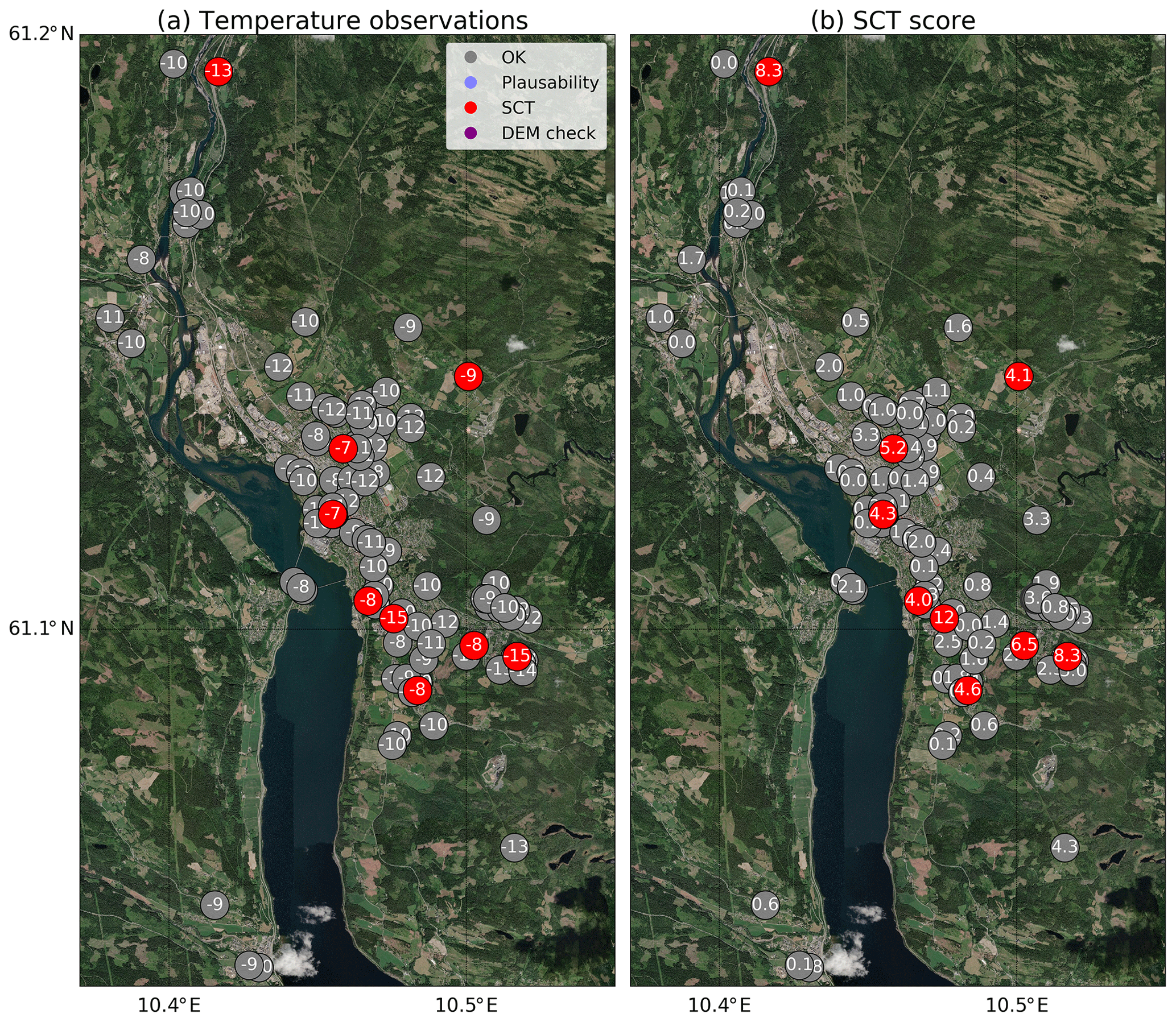
Figure 2 The result of the quality control by Titan for observations in Lillehammer for 06:00 UTC on 5 November 2019, showing the temperature observations (a) with the corresponding SCT scores (b). The observations passing the quality control are shown in grey, whereas those failing the plausibility check, the DEM check, or the SCT are shown in light purple, dark purple, and red, respectively. Background image source: ESRI World Imagery.

Figure 3 shows the temperature and SCT score values for 12:00 UTC on 28 July 2019 for the central part of the city of Oslo, Norway. This case shows a dense observational network with a lot of redundancy, which can be very useful during the summertime when many amateur stations report too high temperatures due to insufficient radiation shielding. The temperature is around 30 ^∘C for this warm summer day. We have around 10 stations flagged from the plausibility check as they show temperature above 40 ^∘C, and two stations are flagged by the DEM check. The rest of the flagged observations are taken out by the SCT, with scores ranging from 4.0 (almost accepted) to around 10.

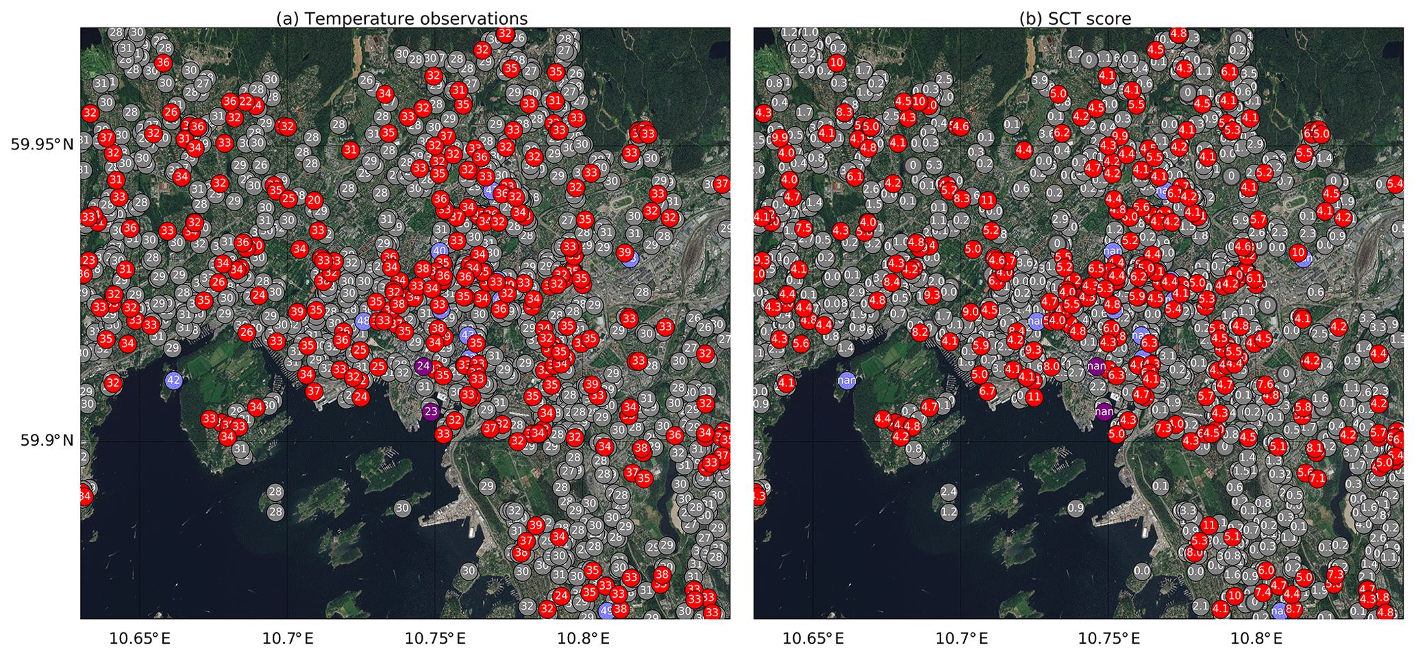
Figure 3 The result of the quality control by Titan for observations in Oslo for 12:00 UTC on 28 July 2019, showing the temperature observations (a) with the corresponding SCT scores (b). The observations passing the quality control are shown in grey, whereas those failing the plausibility check, the DEM check, or the SCT are shown in light purple, dark purple, and red, respectively. Background image source: ESRI World Imagery.

Both examples show the SCT to be the most effective check among those available in Titan, at least when using the current settings. Nipen et al. (2019) found that on average Titan removes 21 % of the measurements, and that the SCT is responsible for about 16 % of that.

3.2 Quality control of hourly precipitation

The plausibility check uses the thresholds of 0 and 100 mm. As for temperature, we are not using any climatological checks.

As discussed in Sect. 2.1, we are cross-checking precipitation and temperature. The temperature data are extracted at the observation locations from numerical model output fields. In this way, each observation of precipitation can be quality controlled, even where the stations are not equipped with temperature sensors. In particular, we use the temperature forecasts from the MetCoOp Ensemble Prediction System (MEPS, Frogner et al., 2019). MEPS has been running operationally four times a day (00:00, 06:00, 12:00, 18:00 UTC) since November 2016. The hourly fields are available over a regular grid of 2.5 km. All the observations of precipitation measured by stations that do not have heated gauges are flagged as suspicious if the corresponding temperature is less than 2 ^∘C.

For the event-based buddy check we have used the condition “greater or equal to” 0.1 mm as the threshold for the distinction between precipitation or no precipitation. Then, the test is applied in two slightly different configurations. For both configurations, we require the same size of 10 km for the square box surrounding each observation, moreover the box must contain at least 10 buddies otherwise the test is not performed. In the first configuration, only in-situ observation are allowed as buddies and an observation is flagged as suspicious if it measures precipitation yes (no) and all the other buddies report precipitation no (yes). In the second configuration, the buddies are searched both within the in-situ observations and among the precipitation estimates derived from the composite of MET Norway's weather radar. An observation is flagged as suspicious when it measures precipitation yes (no) and less than 5 % of the buddies agree with it.

The traditional buddy check is performed over Box–Cox transformed data, as described in Sect. 2.1. As for the buddy event, the test is applied in two slightly different configurations. In the first configuration, only in-situ observations are allowed as buddies. The size of the square box considered is 3 km and the minimum number of required buddies is five. An observation is flagged as suspicious if its distance from the estimated mean, in terms of standardized units, is five times the standard deviation. In the second configuration, the buddies are searched both within the in-situ observations and among the radar data. The size of the square box considered is 5 km and the minimum number of required buddies is 10. An observation is flagged as suspicious if its distance from the estimated mean is seven times the standard deviation.

For both the buddy checks, the event-based and the traditional one, the thresholds have been determined through trial and error experiments. Different priorities have been given to stations, depending on their categories, such that stations in category I have the highest priority, then category II follows, while stations in category III are considered the least reliable. Each check/configuration is iterated until no observations are flagged as suspicious, for a maximum of 10 iterations.

The first-guess check with a deterministic field as the background is implemented checking the in-situ observations against the radar field, where the radar data is available. An observation can be flagged as suspicious in either one of the two situations described below. First, we trust the radar measurements for the distinction between precipitation yes/no. An observed value is suspicious when it is less than 0.1 mm, while the closest radar data value is greater or equal to 0.3 mm. Second, since precipitation errors follow a multiplicative error model (Tian et al., 2013), we expect deviations between radar data and in-situ observations to increase with the precipitation amount. The observed value is suspicious when the closest radar value is greater than 5 mm and the observed value is less than 50 % of the radar value.

For precipitation, the settings for: the first-guess check based on ensemble model output, the SCT and the COOL test are not robust enough to be presented here. At present, we are working on these tests and more efforts are needed to achieve configurations that we feel confident enough to present as examples.

As for temperature, the isolation test is performed after the other tests. Observations not in category I with less than three neighbouring stations within a 25 km radius are flagged as isolated.

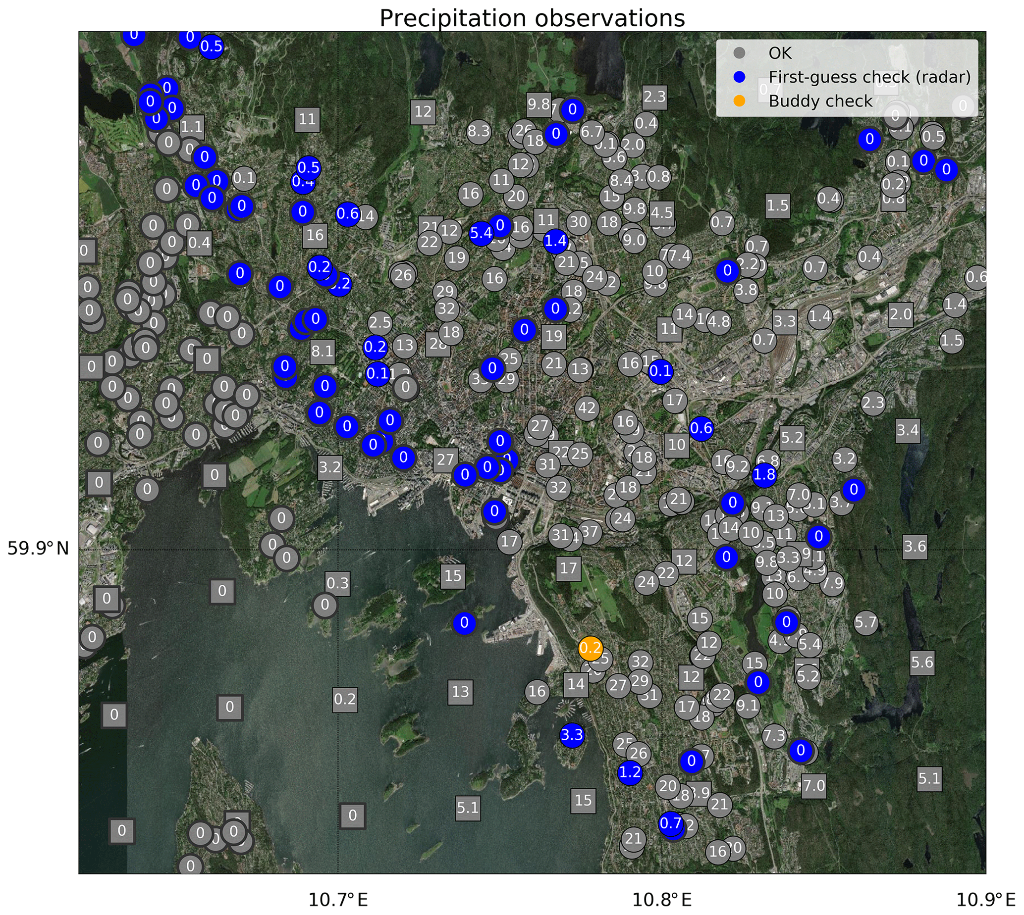
Figure 4 The result of the quality control by Titan for precipitation observations in Oslo for 00:00 UTC on 4 August 2019. The values are total accumulated precipitation over the last hour. The observations (circles) passing the quality control are shown in grey, whereas those failing the buddy check or the first-guess check (radar) are shown in orange and blue, respectively. The radar data are shown as a grid of grey squares. Background image source: ESRI World Imagery.

Figure 4 shows the Titan flags for 00:00 UTC on 4 August 2019 for Oslo, that refers to total precipitation accumulated between 3 August 23:00 UTC and 4 August 2019 00:00 UTC. A thunderstorm was hitting the eastern part of the city, moving from the north to the south of the domain. The narrow north-south band of intense precipitation is clearly visible in the middle of Fig. 4, where it is surrounded by dry regions. The observations are characterized by an extremely large variability over very short distances. For example, the observed values increase from 0 to 42 mm over just a few kilometers in the centre of Oslo. Because of this large variability of the observations this case can be considered a challenging one, and for this reason we have chosen it as an interesting example. Since the season considered is the summer, when temperatures around Oslo are higher than 2 ^∘C, the cross-check is not flagging any observations. The buddy-event check tends also to be more useful in cold weather, when the combined effects of strong winds and low temperatures may cause significant precipitation undercatch also in heated gauges. The traditional buddy check identifies one suspicious observation measuring 0.2 mm that is surrounded by buddies recording much higher values. The test that is flagging all the remaining suspicious observations is the first-guess check with the radar data as the background. There is a substantial agreement between the radar-derived precipitation estimates and the in-situ observations (shown in Fig. 4), nonetheless the values recorded by the two data sources may sometimes differ significantly. The radar dataset considered has a spatial resolution of 3 km. The precipitation system shown in Fig. 4 presents a sharp edge on its west flank where the precipitation values suddenly raise from 0 to 10–20 mm over distances that might be less than 3 km. In this case, some of the in-situ observations reporting 0 mm have been flagged as suspicious because of their deviations compared to the radar background. For some of these observations, we might argue that the first-guess check is flagging good observations as suspicious. The situation is different for observations in the south and in the west of the domain, where the first-guess check is flagging observations that are likely to be suspicious because they report much less precipitation than the first-guess and, at the same time, the pattern of those flags does not seem to reveal any coherent structure related to the characteristics of the precipitation system.

4 Conclusions

The Titan project provides a flexible procedure for the automatic quality control of in-situ meteorological data. In its current form, Titan is a program implementing a sequence of tests mainly focusing on: identifying station locations that may have missing metadata and elevations, identifying non-plausible values using different range checks, and ensuring spatial consistency between nearby observations. The spatial tests are the core of Titan and they include direct comparisons between an observation and its neighbours, or buddies, and the more sophisticated SCT borrowing strength from statistical interpolation methods, such as OI. In addition, Titan facilitates the comparison between in-situ observations and datasets from other data sources, such as numerical model fields and remote sensing.

Titan can be applied to a broad range of near-surface meteorological variables, we have developed and tested it for temperature and we are working on its application to precipitation. In the case of precipitation, some specific tests are available, such as the cross-check between temperature and precipitation and the COOL test. The cross-check test is used to flag non-heated gauges during wintertime, while the COOL test constitutes a practical way to identify non-representative observations.

The presented Titan configuration for temperature is currently used at MET Norway in the production of automatic weather forecast that is delivered on an hourly basis on the popular web-interface https://www.yr.no/.

From a technical point of view, the current version of Titan is written in R (R Core Team, 2015) and the program is made available for public download at https://github.com/metno/TITAN (14 July 2020) with a GNU General Public License v3.0. We are now working on transforming this program into a library of functions that we have named titanlib. The aim is to have the library as a collection of C$++$ functions, which is an ideal choice for the integration into operational applications within national meteorological and hydrological institutes, but with headers that allow using the titanlib functions directly in other languages, such as R or Python. In fact, while working on the development of Titan and presenting our work to colleagues in conferences, we have realized that automatic quality control procedures have been implemented, or are under development, in almost every public or private institute dealing with in-situ observations. Starting from common needs, a large variety of specific solutions can be found because the quality control procedure is often tightly integrated within the particular production chain of each institution. In this sense, Titan being a program may limit its usefulness for other institutes that have different production chains that the one used at MET Norway. Our hope is that titanlib will serve more users, such that a community of people will contribute to it. The strength of a community working on quality control procedure will not be only on the code development, but also on testing the different checks and setting the related thresholds. This last operation is by far the most time consuming task, that ideally should rely on statistics over several years in order to assess the sensitivity of the tests to different thresholds. However, sometimes the number of experiments is limited, especially for those projects where quality control is just an intermediate step and not the final result. A broader assessment of threshold sensitivity must still be done over our observational network and we plan to do it in the near future. As proposed in Sect. 2.1 one could optimize the thresholds by investigating a range of case studies where the results from Titan are compared to the outcome of the quality control from experienced staff checking a subset of the observations. In the future we also plan to integrate titanlib more closely into the wider quality assurance system at MET Norway.

Future developments of the methods in titanlib will include checks of statistics derived from timeseries analysis, such as the check for abrupt variations in the timeseries (step test) and further implementation of the climatological range check for our applications. Timeseries analysis has been ignored in Titan and we recognize this as a limitation of the program that we will remedy in the library.

Another point that is open for development is the decision-making process yielding the final choice on the observation quality. At the moment, we opted for a sequential approach, where each test in the chain inherits information from the previous one and passes only good observations to the subsequent ones. However, an interesting alternative would be to perform several checks in parallel, then comparing their outcomes in terms of “probabilities of having a suspect observation”.