Numerical modelling of the wind over forests: roughness versus canopy drag

Parameterizing the effect of vertically-distributed vegetation through an effective roughness (z_0,eff) – whereby momentum loss through a three-dimensional foliage volume is represented as momentum loss over an area at one vertical level – can facilitate the use of forest data in flow models, to any level of detail, and simultaneously reduce computational cost. Results of numerical experiments and comparison with observations show that a modelling approach based on z_0,eff can estimate wind speed and turbulence levels over forested areas, at heights of interest for wind energy applications (∼60 m and higher), but only above flat terrain. Caution must be exercised in the application of such a model to zones of forest edges. Advanced flow models capable of incorporating local (distributed) drag forces are recommended for complex terrain covered by forest.

1 Introduction

Comprehensive investigation is needed to estimate the wind energy potential at any given site. Along with field measurement campaigns, different kinds of models are widely used nowadays. For sites of moderate or high complexity, RANS (Reynolds-Averaged Navier-Stokes) solvers have become a commonly-used tool in the wind energy industry (e.g. Sørensen et al., 2017). Increasing detail in the description of the site in the RANS model, along with improving the quality of the model, tends to increase the computing cost. Trees present at the site add a level of complexity to wind flow modelling. Due to rapid technological improvement in airborne lidar scanning (ALS), data on land surface and vegetation characteristics have become available, with increasing detail and quality. Methods have been developed to allow calculation of highly heterogeneous and realistic Plant Area Density (PAD) using raw ALS data (Lefsky et al., 1999; Richardson et al., 2009; Boudreault et al., 2015). To facilitate usage of ALS forest data in flow models with different types or levels of canopy drag-force prescription (e.g. linearized, RANS, and mesoscale models), Sogachev et al. (2017) recently suggested an objective method to translate PAD (momentum absorbed mostly by foliage distributed in the vertical) into spatially varying values of effective roughness, z_0,eff (momentum absorbed at one vertical level). The effective roughness can be used to connect the surface friction velocity and geostrophic wind speed in a way satisfying the geostrophic drag law (Blackadar and Tennekes, 1968); it also allows prediction of wind flow over vegetation using typical numerical models, without needing to incorporate local drag forces in each grid volume of a three-dimensional model domain (see Fig. 1). In the present study, we explore the effect of different canopy representations on flow modelling over two forested sites: one located on a flat coastal plain (Østerild, Denmark) and the other in a hilly region (Rödeser Berg, Germany).

Figure 1 Schematic of principles behind (a) the drag force and (b) the roughness height (adapted from Boudreault, 2015).

2 Modelling

2.1 Models

Forests significantly reduce wind speeds and increase turbulence intensity. To address this, DTU Wind Energy has been developing RANS parameterizations for drag-induced effects of vegetation for many years. The atmospheric boundary layer (ABL) model SCADIS (Sogachev et al., 2002, 2012), based on a finite-difference numerical approach, is a basic tool for investigation of vegetation effects on atmospheric flow. Due to its flexibility, SCADIS allows testing of any assumption in a straightforward way. However, the model was designed for a single processor and cannot yet be used on the massive computing scale, needed for the wind industry. However, DTU Wind Energy's other in-house RANS (finite-volume) solver, EllipSys3D (e.g. Michelsen, 1992; Sørensen, 2003), was programmed for massively parallel computing, though it was not designed for the ABL. Based on fundamental investigations and research using SCADIS, EllipSys3D has been improved in order to simulate forested ABL flow problems. Both RANS models apply the two-equation closure approach based on coupled transport equations for the turbulent kinetic energy (TKE) k, and a supplementary length-scale determining variable φ (which can be e.g. ε or ω, where ε is the dissipation rate of TKE and $\mathit{\omega }\equiv \mathit{\epsilon }/k$) (e.g. Pope, 2000).

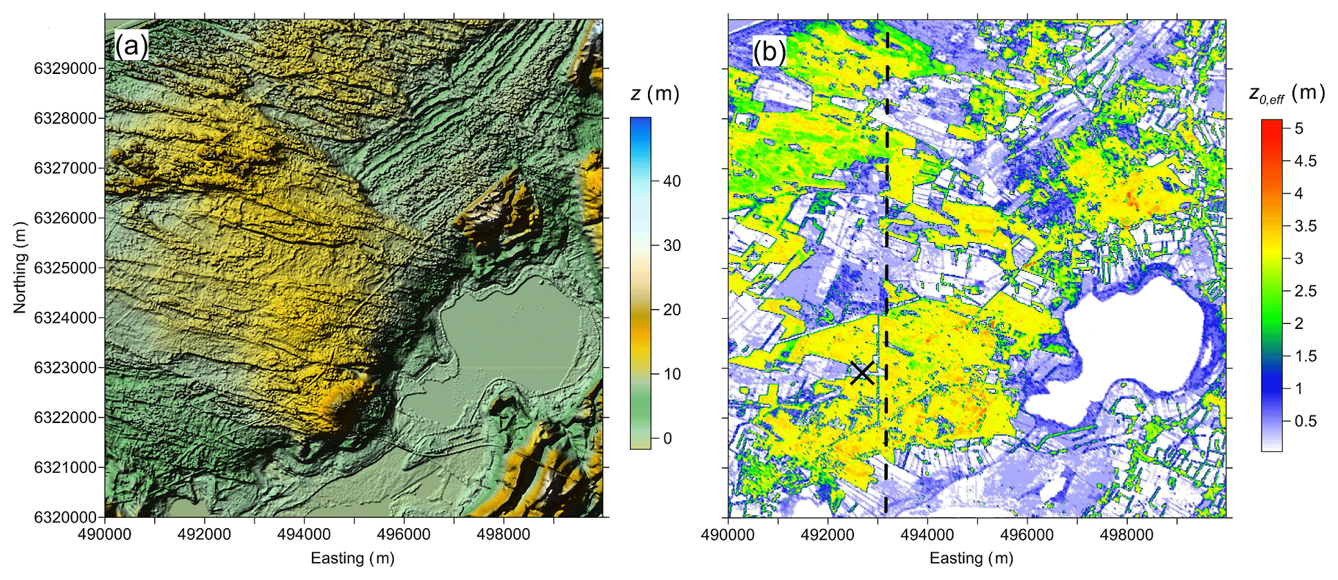
Figure 2 (a) Shaded relief plot of the elevation and (b) horizontal distribution of modelled effective roughness, z_0,eff, at Østerild. Elevation map was produced using freely available data from Styrelsen for dataforsyning og effektiviseri , DHM-2007/Terræn (1.6 m grid) (DHM – Danmarks Højdemodel, http://download.kortforsyningen.dk, last access: June 2019). The calculation resolution is 16 m ×16 m. Cross indicates the location of measuring tower. Dashed line indicates transect used for modelling results presented in Fig. 5.

Figure 3 (a) Shaded relief plot of the elevation, and (b) horizontal distribution of modelled effective roughness, z_0,eff, at Rödeser Berg. Elevation map was produced using data derived by Freier (2017) from ALS data set available from the Hessian Administration Office of Land Management and Geological Information (HVBG, 2010). The calculation resolution is 10 m ×10 m. Cross indicates the location of measuring tower. Dashed line indicates transect used for modelling results presented in Fig. 8.

2.2 Vegetation description in models

In the models with canopy drag-force prescriptions, detailed information about PAD can be directly used after modification of the RANS equations. Modification usually includes additional terms in the momentum and turbulence closure equations:

1. in the momentum (or velocity) component equations, for each spatial coordinate (direction) x_i, the grid-volume average momentum sink of canopy elements is usually parameterized by Raupach and Shaw (1982)

   $$\begin{array}{}\text{(1)}& F_i=-c_{\mathrm{d}}\mathrm{PAD}\langle {\stackrel{\mathrm{‾}}{U}}_i\rangle S.\end{array}$$

   Here $S=(\langle {\stackrel{\mathrm{‾}}{U}}_i\rangle \langle {\stackrel{\mathrm{‾}}{U}}_i\rangle {)}^{\mathrm{1}/\mathrm{2}}$ is the magnitude of the spatial (angle brackets) and temporal (overbar) average of the wind speed, and c_d is the drag coefficient including the shelter effect.

2. In the turbulence closure equations (i.e. for k and φ), a wake production term and enhanced dissipation term due to the surface drag of canopy elements (e. g. Raupach and Shaw, 1982; Finnigan, 2000) is added. In contrast with conventional parameterizations for vegetation-induced momentum sinks, modification of the closure equations is still debated somewhat. In the present study, we use the canopy parameterizations described in Sogachev et al. (2012, 2015).

With an effective roughness approach, no modification of the RANS equations is needed; use of z_0,eff allows us to predict airflow over a (displaced) surface covered by the vegetation using a flow model, without explicitly resolving the canopy drag. A method for deriving z_0,eff from frontal area density consists of three basic steps (Sogachev et al., 2017):

1. using a statistical approach to rank frontal density data into land-use classes;

2. applying empirical methods to describe the mean properties (per each class):

3. utilizing the RANS solver to estimate the aerodynamic roughness, z_0,eff and as such to effectively describe each land-use class with a single parameter.

The SCADIS model using k-ε closure is employed in the last step here. SCADIS provides steady-state profiles of velocity components, turbulent kinetic energy, dissipation rate and the mean momentum flux for a specified geostrophic wind G, Coriolis parameter (i.e. latitude), and predefined canopy drag. Thus, a “geostrophic drag law” (e.g. Blackadar and Tennekes, 1968) is implicitly applied, which, combined with Rossby number similarity theory, gives the following geostrophic wind in the neutral, barotropic boundary layer:

$$\begin{array}{}\text{(2)}& G={\displaystyle \frac{u_{\ast ,\mathrm{0}}}{\mathit{\kappa }}}{\left[{\left(\ln {\displaystyle \frac{u_{\ast ,\mathrm{0}}/f}{z_{\mathrm{0},\mathrm{eff}}}}-A\right)}^{\mathrm{2}}+B^{\mathrm{2}}\right]}^{\mathrm{1}/\mathrm{2}}.\end{array}$$

Thus

$$\begin{array}{}\text{(3)}& z_{\mathrm{0},\mathrm{eff}}={\displaystyle \frac{u_{\ast ,\mathrm{0}}}{f}}\exp \mathit{\{}-\left[{\left({\left({\displaystyle \frac{\mathit{\kappa }G}{u_{\ast ,\mathrm{0}}}}\right)}^{\mathrm{2}}-B^{\mathrm{2}}\right)}^{\mathrm{1}/\mathrm{2}}+A\right]\mathit{\}}.\end{array}$$

In Eqs. (2) and (3) κ is the von Kármán constant (usually accepted to be 0.4), f is the Coriolis parameter, $u_{\ast ,\mathrm{0}}$is the friction velocity at the “virtual” surface (generally the mean tree-top height). The geostrophic component coefficients A, B have historically been established empirically via ABL measurements (Melgarejo and Deardorff, 1974; Clarke and Hess, 1974). Our calculations used A=1.8 as in Troen and Petersen (1989) and wind energy practice (roughly equal to the mean of values found in literature). The value B=6.4 is fitted to match solutions of SCADIS with drag forces and z_0,eff and is slightly higher than the value B=4.5 given by Troen and Peterson (1989). In all calculations, G is taken as 15 m s⁻¹ and f is specified in accordance to the location of the test site (see below).

2.3 Numerical experiments

The RANS solver EllipSys3D, which uses a k-ε turbulence model, was applied for numerical simulation of the wind field. For the present simulations, a polar (cylindrical) computational domain is chosen. The two main reasons for selecting a cylindrical domain are that the finest grid resolution is provided at the central part of the domain where it is most needed, and that the solution mesh is equally suited for ?ow from all directions. In the central part of the domain, a square grid zone is used around the target area. For both sites, the computational domain has a radius of about 25 km and a height of about 5 km. The target area for Østerild is about 10 km by 10 km with a horizontal resolution of 16 m (see below). The target area for Rödeser Berg is about 8 km by 8 km with a horizontal resolution of 10 m (see below). The vertical grid consists of nodes with variable size (i.e. about 1 cm near the ground and with maximal vertical resolution of 1 m in first 50 m above ground) allowing the canopy drag to be properly resolved. Details about modelling of complex terrain flow using EllipSys3D can be found in Koblitz (2013) and Sørensen et al. (2017). Calculations were done for the neutral flow using a steady-state algorithm for three geostrophic wind directions for Østerild site (90, 200, and 290^∘) and one geostrophic wind direction (210^∘) for Rödeser Berg site both with a full description of canopy drag forces and with forest replaced by the effective roughness. Note that wind direction in the surface layer is turned in respect to the geostrophic wind direction by approximately 20^∘ counter clockwise. Thus, modelled surface wind directions are circa 70, 180, and 270^∘ for Østerild site and circa 190^∘ for Rödeser Berg site. In these calculations, G is taken as 15 m s⁻¹, to provide calculated wind speed magnitude in surface boundary layer closer to that observed here.

Figure 4 Normalized observed (circles) and modelled (lines) wind speed profiles at the mast position in Østerild site for different wind directional sectors around (a) 70^∘, (b) 180^∘ and (c) 270^∘. Modelled results plotted for the case with a full description of canopy drag forces (black) and the case with forest replaced by the effective roughness (red). Bars denote standard deviations normalized on S₂₄₀.

3 Sites

3.1 Østerild site

The Østerild site is located on a coastal plain, in northern Jutland, Denmark. Figure 2a shows that the terrain is flat, except for a small hill in the southwest direction and some sand dunes to the north. The site has grasslands, and forests with scotch pine, mountain pine, silver fir, Sitka spruce, oak, and birch. Most of the tree heights are between 15 and 20 m. The PAD for this site was derived from ALS data using the method of Boudreault et al. (2015). Figure 2b shows the estimated values of effective roughness over the target domain. The original elevation data set had a horizontal resolution of 1.6 m. To demonstrate the method and to speed up data processing, here we use a resolution of 16 m. There are multiple sets of observational data from the Østerild site, but only data derived from the 250 m tall met mast equipped with sonic anemometers at 5 height levels (for detail see Peña, 2019) are used in this study. The selection of date was done following Dellwik et al. (2014) recommendations.

3.2 Rödeser Berg site

The Rödeser Berg site is located in central Germany (in the northern part of the federal state of Hesse). Figure 3a shows that the terrain in this area is hilly, with the elevation reaching from 200 to 500 m. The forest type at the Rödeser Berg is a mixed forest, consisting mainly of beech trees, pine trees, and spruces, with a few areas of larch and oak. Less than 1 % of the trees in the area are taller than 40 m, and most of the trees have heights between 25 and 32 m. There are several clearings, forest roads and some scattered houses close to the forest edges. Details about ALS data and how PAD values were produced for this area are given in (Freier, 2017). Figure 3b shows the estimated values of effective roughness over the target domain. There are several met measurement facilities on this site (for detail see Mann et al., 2017). Only data from the 200 m tall met mast equipped with sonic anemometers at 9 height levels and located at the top of Rödeser Berg are used in the current study. Relatively few cases were selected, and the sample size was too small for reliable uncertainty estimates.

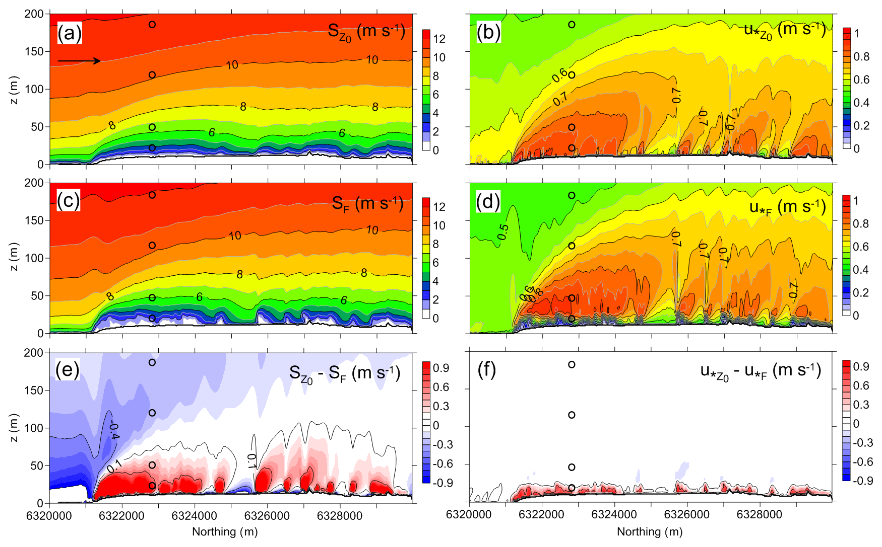
Figure 5 Two-dimensional fields of (a, c) wind speed (S) and (b, d) local friction velocity (u_∗) along the south-north transect (see location in Fig. 2b) modelled by EllipSys3D using the effective roughness (subscript z₀) and the canopy drag (subscript F) approaches. The differences in values of S and u_∗ derived using two different approaches are also shown in (e) and (f), respectively. Arrow in (a) shows the flow direction. Thick black lines in panels indicate the surface. Open circles in panels indicate observation points.

4 Results

4.1 Coastal plain

Figure 4 compares the normalized wind speed profiles derived from measurements with numerical simulations, for the mast position at Østerild. Measured data are presented for the directional sectors of 30^∘ wide closest to modelled wind directions. Figure 4 demonstrates the model's ability to qualitatively reproduce wind speed over the forested area. Good agreements between modelled data and observations are noted for easterly (Fig. 4a) and southerly (Fig. 4b) winds. For westerly winds (Fig. 4c), the RANS simulations provide wind speed profiles laying between those that were observed for two adjacent wind sectors. A possible reason for the scatter in observations with wind direction is the large clear-cut, W/SW of the mast (see Fig. 2b). A minimal difference in wind speed profiles is found between the two different canopy approaches for easterly winds; this is probably because the longest forested fetch exists towards the east (see Fig. 2b). Small differences in wind speed profiles derived by the canopy approaches for southerly and westerly winds can be explained by the presence of clear-cuts of different sizes, and limited fetch. In both cases, the difference in data derived by two approaches decreases for heights farther above the ground. No difference is observed above a height of ∼100 m.

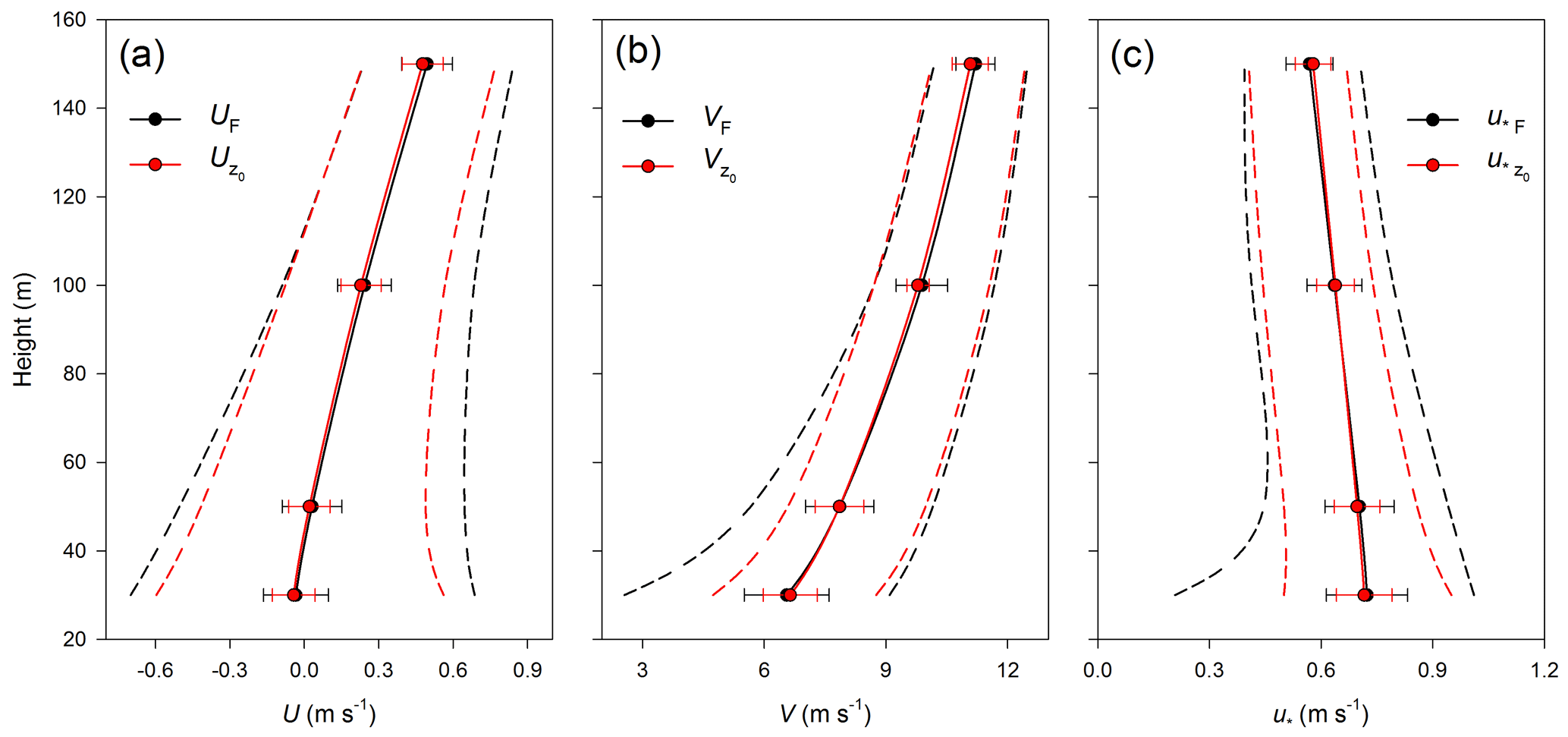
Figure 6 Average values of (a) eastward (U) and (b) northward (V) components of wind speed and (c) local friction velocity (u_∗) in the area of interest at different heights over ground (30, 50, 100 and 150 m) derived using the canopy drag (black) and the effective roughness (red) approaches. Bars denote standard deviations. Range of variables is indicated by dashed lines.

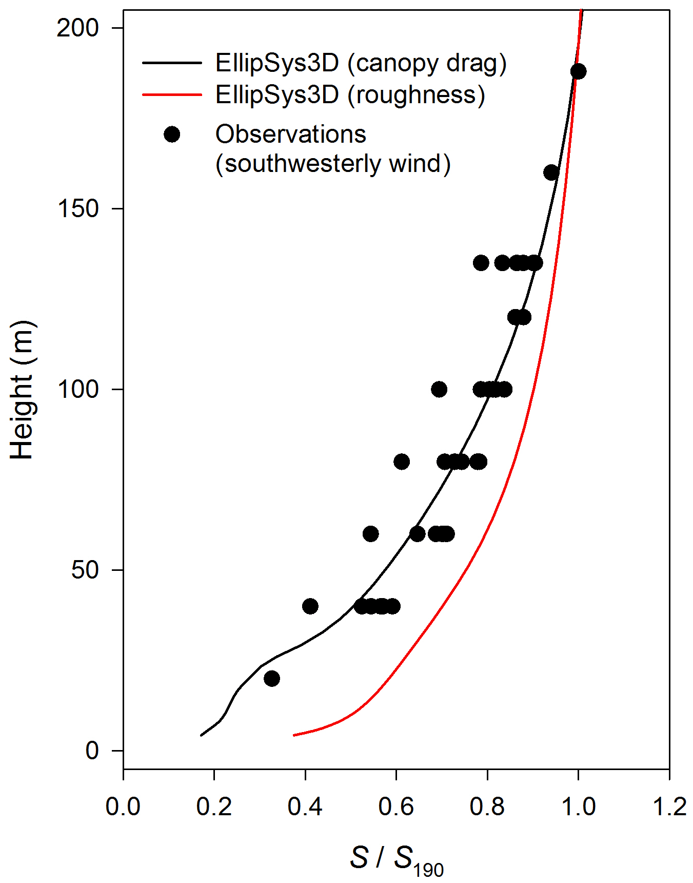
Figure 7 Normalized observed (circles) and modelled (lines) wind speed profiles at the mast position in Rödeser Berg site for wind direction sector around 190^∘. Modelled results plotted for the case with full description of canopy drag forces (black) and the case with forest replaced by the effective roughness (red).

Figure 5 shows wind speeds (S) and local friction velocity (u_∗) along the north-south transect over the area indicated in Fig. 2b (dashed line), modelled using the two canopy approaches for southerly winds. The results of the numerical experiments presented in Fig. 5 show that models with different parameterization of the vegetation effect produce similar wind speeds (Fig. 5a, c) and local friction velocities (Fig. 5b, d) over the investigated domain. The effects of vegetation on the airflow are clearly seen. When using the canopy drag parameterization, the model provides more details on airflow near the ground, but with increasing the height flow parameters become smoothed. One can see that the large difference in estimated wind speed fields (Fig. 5e) as well as in estimated local friction velocities (Fig. 5f) is observed in the lowest layer of atmosphere and of course inside the layer occupied by vegetation. Data presented in Fig. 5e indicate that the largest difference in wind speed occurs in the zones of forest edge, especially when the wind hit the forest from an open place with large upwind fetch.

To exclude the local effect of the underlying surface on wind profiles we consider average values of flow parameters over Østerild target area at different heights. Figure 6 shows that the model with the different parameterizations of the vegetation effect produces similar results, except the effective roughness approach provides a smaller scatter of modelled variables around its average value.

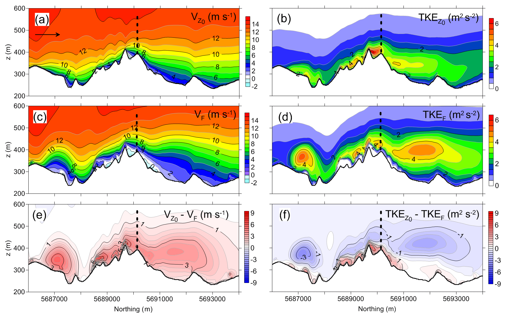
Figure 8 Two-dimensional fields of (a, c) northward component of wind speed (V) and (b, d) turbulent kinetic energy (TKE) along the south-north transect (see location in Fig. 3b) modelled by EllipSys3D using the effective roughness (subscript z₀) and the canopy drag (subscript F) approaches. The differences in values of V and TKE derived using two different approaches are also shown in (e) and (f), respectively. Arrow in (a) shows the flow direction. Thick black lines in panels indicate the surface. Dashed lines in panels indicate the met mast position.

Figure 9 Average values of (a) eastward (U), and (b) northward (V) components of wind speed and (c) turbulent kinetic energy (TKE) in the area of interest at different heights over ground (30, 50, 100 and 150 m) derived using the canopy drag (black) and the effective roughness (red) approaches. Bars denote standard deviations. Range of variables is indicated by dashed lines.

4.2 Hilly terrain

Figure 7 compares the normalized wind speed profiles derived from measurements and numerical simulations at the mast position at the Rödeser Berg site. Observed data are scattered because they are for different wind directions inside the southwestern sector (180–225^∘). The model does a good job in reproducing the wind speed profile with the canopy drag prescription approach, but fails with the effective roughness approach. Figure 8 shows results along the north-south transect over the area indicated in Fig. 3b (dashed line) modelled using different canopy approaches for the southern wind sector. One can see that the two canopy model implementations give similar airflow only upwind of the hill; on the summit and downwind, the modelled airflow structures are different. The approach based on effective roughness results in higher wind speed (Fig. 8a, see also Fig. 7) above topographic peaks, in comparison with the full drag approach (Fig. 8c, e). The roughness-based approach overestimates TKE values (consideration of the local friction velocity in our opinion has limited quantitative value regarding complex terrain flow) near the ground (again especially at topography summits), but underestimates TKE values at higher altitudes, and especially downwind of topography summits (Fig. 8b, d and f). Analysis of average values of flow parameters over Rödeser Berg target area at different heights (Fig. 9) retrievals that the roughness model approach in general provide higher wind speed (Fig. 9a, b) and lower TKE levels (Fig. 9c) than provided by the full drag model approach. The roughness model approach also provides a narrow scatter of modelled variables around its average value.

5 Conclusions

Targeted numerical experiments and their comparison with observations indicate that using a roughness representation of forest within typical RANS flow modelling, one can estimate wind speed and turbulence levels over forested areas, at heights potentially interesting for wind energy applications (∼60 m and higher) – but only above the flat terrain. Not surprisingly, the roughness-based approach becomes less valid near forest edges, and more valid in directions with longer forest fetch; for the former limitation, there is consistency between our results and the linearized modelling attempts made by Bingöl (2010). Advanced flow models capable of incorporating (distributed) local drag forces are recommended for complex terrain covered by forest, and the RANS turbulence model likely needs to be extended to predict flow over hilly forested terrain.