 | 21 Apr 2021
Raindrop fall velocity in turbulent flow: an observational study
Merhala Thurai
Viswanathan Bringi
Patrick Gatlin
Mathew Wingo
Laboratory measurements of drop fall speeds by Gunn–Kinzer under still air conditions with pressure corrections of Beard are accepted as the “gold standard”. We present measured fall speeds of 2 and 3 mm raindrops falling in turbulent flow with 2D-video disdrometer (2DVD) and simultaneous measurements of wind velocity fluctuations using a 3D-sonic anemometer. The findings based on six rain events are, (i) the mean fall speed decreases (from the Gunn–Kinzer terminal velocity) with increasing turbulent intensity, and (ii) the standard deviation increases with increase in the rms of the air velocity fluctuations. These findings are compared with other observations reported in the literature.
- Article
(4880 KB) - Full-text XML
- BibTeX
- EndNote


Measurements of the terminal fall speed of drops by Gunn and Kinzer (1949) under laboratory conditions with the pressure correction of Beard (1976) has been the “gold” standard since 1949. Time and again the raindrop (terminal) fall speed (Vt) versus diameter (D) relation based on modern instruments have been shown to follow the Gunn–Kinzer relation (to within the measurement errors) when the conditions are calm (Bringi et al., 2018). However, under windy or turbulent conditions the fall speed for a given drop diameter (D) will not be unique and has to be treated as a distribution where the mean fall speed can deviate from Gunn and Kinzer (1949), termed sub-terminal or super-terminal when the mean fall speed is 30 % less or greater than, respectively, Gunn–Kinzer (Montero-Martinez et al., 2009). In addition, the distributions show finite dispersion and (at times) the shape can exhibit skewness. A number of articles, for example Thurai et al. (2013), Larsen et al. (2014), Montero-Martinez and Garcia-Garcia (2016), Yu et al. (2016), and Bringi et al. (2018) are largely observationally-based, documenting conditions that sub- or super-terminal fall speeds occur. The mechanisms are not clear, but sub-terminal velocity after a collision-coalescence event (tiny drop collides with large drop which “slows” down after coalescence) and the super-terminal velocity after breakup (the smaller drop fragments tend to have the same fall speed as the parent drop) have been proposed. The latter mechanisms depend on the collision frequency, and after a transient period of several 100 ms the drops recover to their terminal fall speeds (Szakáll et al., 2010). To put this in perspective, the mean time between collisions for a 2 mm (3 mm) drop with any other sized drop is around 10 s (3 s) at rain rate of 50 mm h−1 (McFarquhar, 2004).
Table 1Formulas for estimating the relevant quantities.
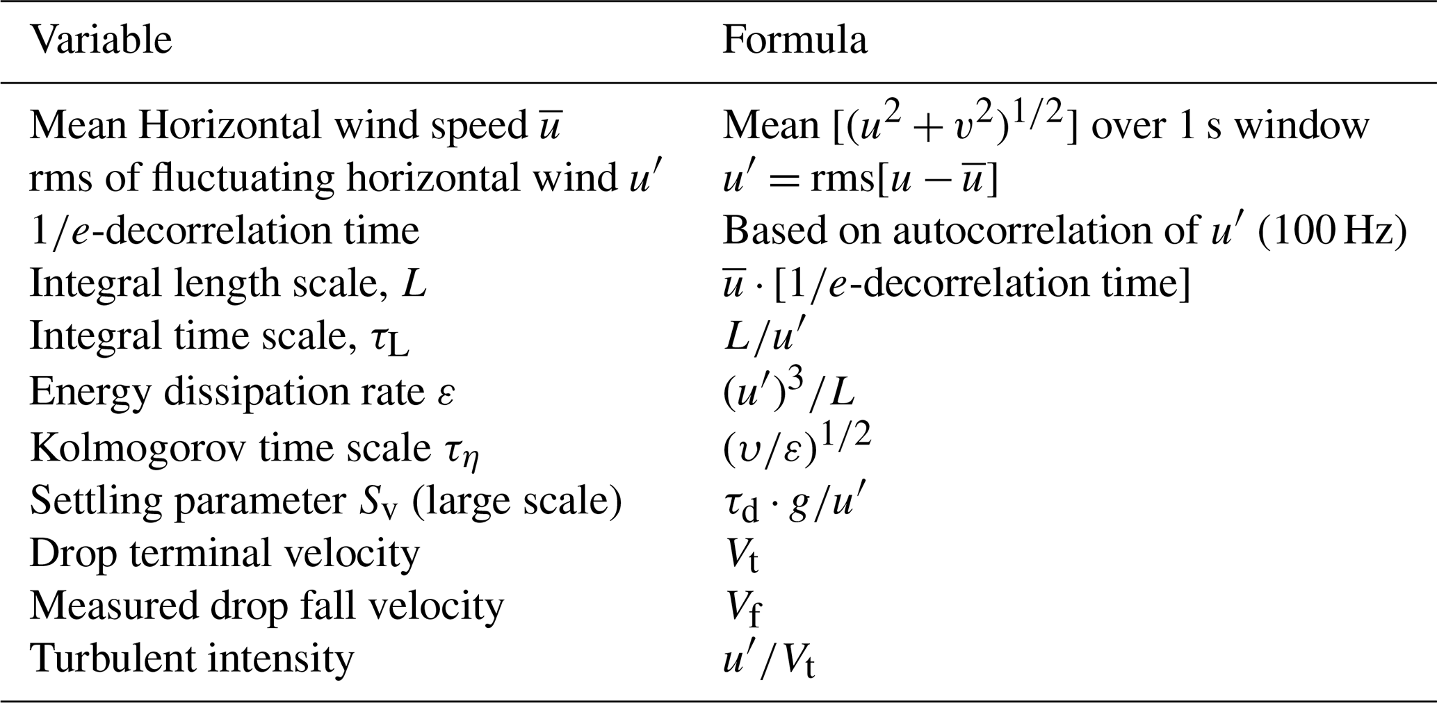
Note: normally the streamwise mean velocity and fluctuations are used.
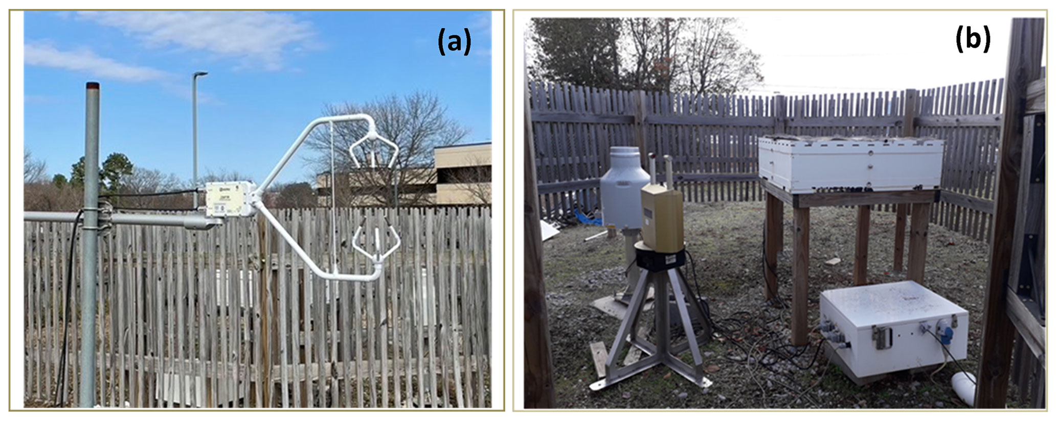
Figure 1Close-up pictures of (a) the 100 Hz sonic anemometer (outside the wind-fence, upwind) and (b) 2DVD:SN16 (inside the double fence), together with Pluvio gauge and other instruments. Note, there is another 2DVD (SN72) outside the double fence a few meters away.
The mechanism most likely for (non-transient) sub-terminal fall speeds (that we consider herein) is turbulence. The early studies of Stout et al. (1995) predicted that mean settling velocity of rain drops modelled as rigid spheres in homogeneous isotropic turbulence (HIT) would decrease (from terminal) depending on turbulent intensity and the Reynolds number (Re) but did not predict the enhanced dispersion of the fall speed distribution (observed by Bringi et al., 2018). The recent article by Ren et al. (2020) uses direct numerical simulation (DNS) to study the drop dynamics of 2 and 3 mm sizes in turbulent flow. Their conclusion was that both sized drops showed a decrease of the mean fall speeds (settling speeds) relative to terminal by 5 %–7 %. for turbulent intensity of 10 % (; see Table 1). One application is related to deriving the drop size distribution from the Doppler spectrum measured by vertical pointing radar for which the terminal fall speed versus drop diameter relation is needed and fits to the Gunn–Kinzer are universally used (e.g., Williams and Gage, 2009). Another application is the numerical solution of the stochastic coalescence-breakup equation where the gravitational kernel involves the terminal fall speeds of the different sized drops that are assumed to follow fits to Gunn–Kinzer (e.g., Morrison and Grabowski, 2006).
In this paper, we present experimental results of measured fall speeds and turbulence-related parameters. Instrumentation and experimental set up are given in Sect. 2; brief background on the parameters/scales of turbulent flow are given Sect. 3; fall speed results for 2 and 3 mm sized drops in varying turbulent intensities are given in Sect. 4, followed by conclusions in Sect. 5. The results reported here provide an extension to our previous study by Thurai et al. (2019).
The principal instruments used in this study for fall speed measurements are two 2D-video-disdrometers (Schönhuber et al., 2007, 2008), one 2nd generation (low profile) unit (SN16) located inside a -scale Double Fence Intercomparison Reference (DFIR; Rasmussen et al., 2012) wind shield (Fig. 1), and one 3rd generation (compact) unit (SN72) a few meters outside the fence. The height of the outer and inner wind-fences are 2.4 and 2 m respectively. The measurement site is located at the University of Alabama in Huntsville (UAH). We have compared the fall speed distributions from (SN16) sited inside the DFIR and SN72 sited ∼5 m outside the DFIR for one rain event (12 July 2020) under conditions of turbulent flow. The histograms of fall speeds from these two instruments are shown in Fig. 2. The histogram shapes are very close with similar modes and width. This implies that the DFIR-induced effects did not change the environmental turbulent flow at the sensing area. Thus the inference can be made that the sonic measured data are representative of the turbulence experienced by the raindrops falling in the sensor area. A research-grade 3D-sonic anemometer (model CSAT3B from Campbell Scientific) is used to characterize the turbulent flow and is sited 3 m upwind from the DFIR (outside). The sampling rate is selectable but for our purposes it was set at the maximum rate of 100 Hz. A standard anemometer at 10 m height sampling at 0.2 Hz was also available. The sonic anemometer measures the 3 wind components, and the sonic temperature. Regular checks of data from the sonic anemometer were performed by comparing with data from the 10 m wind sensor. An example from 23 April 2020 is shown in Fig. 3 where the mean horizontal wind speed at 10 m height (standard anemometer sampling 0.2 Hz) is compared with the sonic anemometer at 1.5 m (sampling at 100 Hz). The mean wind speed (Fig. 3a) over 3 min window and the maximum value (Fig. 3b) in this window were calculated from both instruments. The high correlation between the 10 and 1.5 m mean wind speed and the corresponding maximum values is clearly evident. We can then infer that the turbulence measurements made by the sonic anemometer is largely unaffected by the perturbation due to the presence of the DFIR. Thériault et al. (2015) using Computational Fluid Dynamics software documented in detail the airflow (streamlines) in the vicinity of the DFIR as well as inside the DFIR for two situations: (a) the flow is along the vertex of the octagon and (b) the flow is along the “flat” side (22.5∘) of the octagon. One of their main conclusions is that the flow field described in (a) gives rise to weak updrafts (<0.2 m s−1) at sensor height and (b) weak downdrafts (−0.2 m s−1). Since the flow field can be from any direction the weak vertical air motions would probably be less than m s−1. Thus, in the simulations of Thériault et al. (2015) the DFIR under steady flow does not result in turbulent eddies inside the DFIR, or in other words the sonic anemometer data can be used for estimating the flow parameters with relatively minor influence of the DFIR itself. Further, Zhang et al. (2016) studied the effect of rainfall on the sonic anemometer measurements of wind speeds and found negligible errors introduced by 3 min rain rates up to 50 mm h−1.
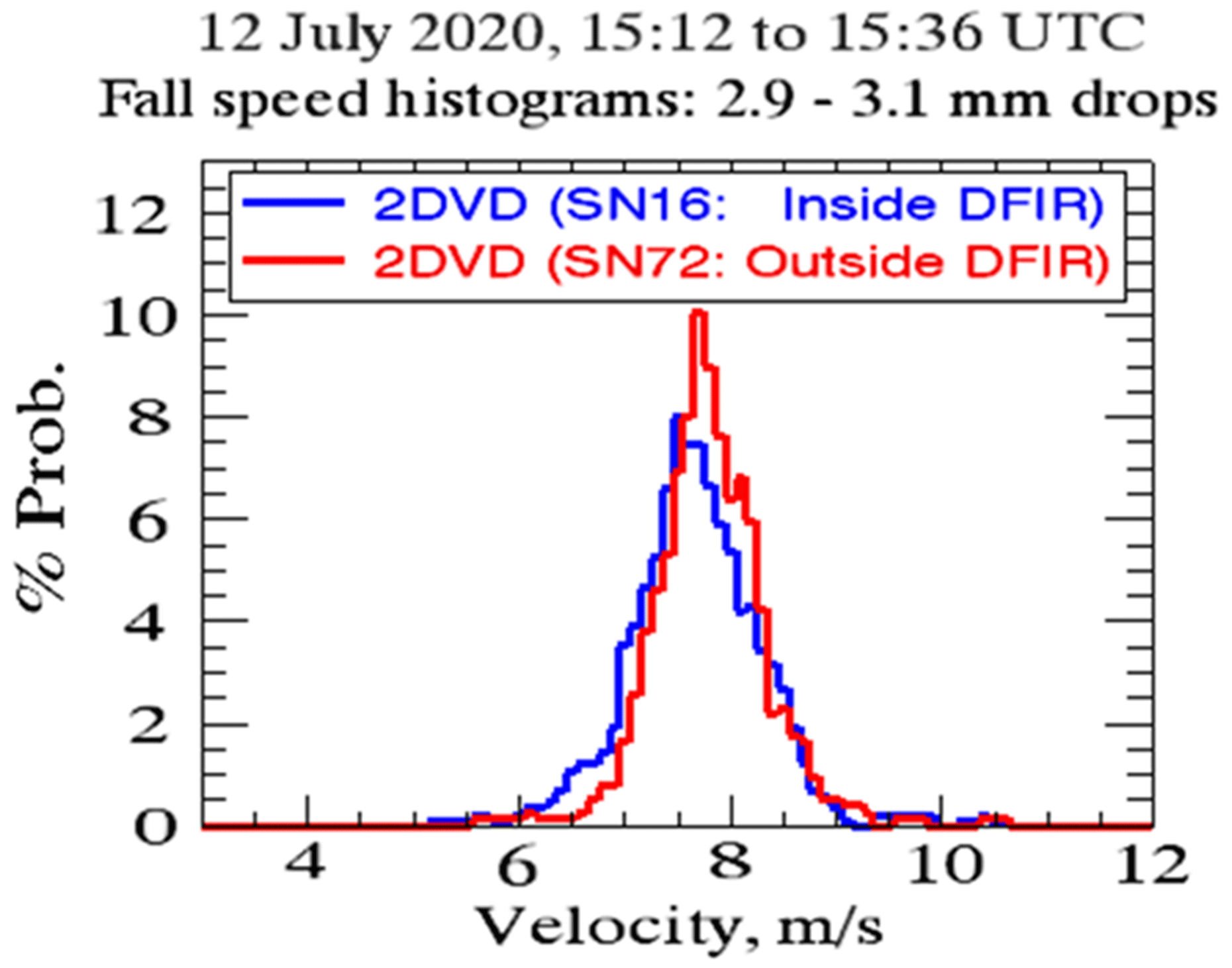

Figure 3(a) Mean wind speed from standard anemometer at 10 m height compared with the sonic aenomometer at 1.5 m. The averaging window is 3 min. (b) As in (a) except the maximum wind speed is shown. The high frequency sonic anemometer data were degraded to match the standard anemometer.
Six rain events with substantial numbers of 2 and 3 mm sized drops were chosen for this study: (i) a small but intense isolated rain cell which traversed the instrumentation site on 8 April 2020; (ii) a relatively larger, mesoscale system with an embedded line convection on 9 April 2020; (iii) pre- and post-frontal precipitation associated with a mid-latitude cyclone traversing the region on 23 April 2020; (iv) a detached rain-cell fragment with high rain intensity on 3 June 2020; (v) part of tropical storm Cristobal on 9 June 2020; and (vi) a widespread event with embedded (highly) convective rain cells on 12 July 2020.
The literature on turbulence in the atmospheric surface layer is vast (e.g. Kaimal and Finnigan, 1994) and it is not our intention to go in any depth on accurate characterization of the flow parameters. Our goal is restricted to observations of the fall speeds (settling speeds) of 2 and 3 mm-sized raindrops falling in the turbulent surface layer. Turbulent flow is described by the large (or, integral) scale eddies with a length scale (L) and a time scale termed as the eddy turnover time. The turbulent kinetic energy at these scales cascades at the eddy dissipation rate (ε) to the smallest scale eddies (the Kolmogorov scale). Our procedure for computing the integral length scale and the eddy dissipation rate follows Nemes et al. (2017) who made the first measurements of the fall speeds of snowflakes in the turbulent surface layer. The basic steps for inferring L and ε, and hence Kolmogorov scales are, (i) measuring the mean horizontal wind speed and rms velocity fluctuations (u′) in a time window of 60 s (at 100 Hz sampling this gives 6000 samples), (ii) computing the autocorrelation of u′ from the 6000 samples, (iii) estimating the -decorrelation time from the autocorrelation of u′ – (i) to (iii) are thus based on successive 6000 samples covering the duration of an event –, (iv) use the Taylor hypothesis to compute L as the product of the -decorrelation time and the 1 min mean horizontal wind speed, and (v) invoking the inertial-dissipation method (Kaimal and Finnigan, 1994; Grachev et al., 2013) under the homogeneous isotropic turbulence (HIT) assumption, to arrive at Table 1, which summarizes the formulas used herein. Time interpolation was performed to extract the values of the necessary parameters corresponding to the timestamp of the specified drops from the 2DVD measurements.
Figure 4 shows the time series of the turbulence scales listed in Table 1 which are available at 1 min resolution. Figure 4h shows the fall speed of 3 mm sized drops (2.9–3.1 mm) from the 2D-video disdrometer (2DVD). An isolated rain cell traversed over the instrumented site at 23:45 UTC for about 15 min. The majority of drops have fall speeds that are lower than terminal velocity, which is close to 8 m s−1 (dashed green line). From Fig. 4a–g the following points can be made. The turbulent intensity () in Fig. 4c reaches a maximum of 0.6 at 23:45 UTC which is among the higher values recorded in our dataset of 6 events. Prior to the rain cell passage the intensity drops to near 0 at 23:30 UTC and generally the ceiling is 0.2. The integral length scale L is much larger than computed by Nemes et al. (2017) who estimated L as 4 m in quasi-stable night time surface layer. The integral time scale which is the ratio of L and u′ is approximately 15 s at 23:45 UTC. The drop response time (; Good et al., 2014) for 3 mm drop is 0.8 s. From Fig. 4e, the Kolmogorov time scale is nearly three orders of magnitude smaller than the drop response time. On the other hand, Nemes et al. (2017) calculated the response time of low density snow particles (mean size of 1 mm and density estimated as 0.05 g cc−1) as 50 ms which is much smaller than the Kolmogorov time scale (τη=0.1 s). This contrast reflects the low snow-to-fluid density ratio and Nemes et al. (2017) experimentally found that the snow particles' mean settling velocity in turbulence was nearly twice the terminal velocity in still air (termed as a “preferential sweeping” mechanism; Wang and Maxey, 1993).
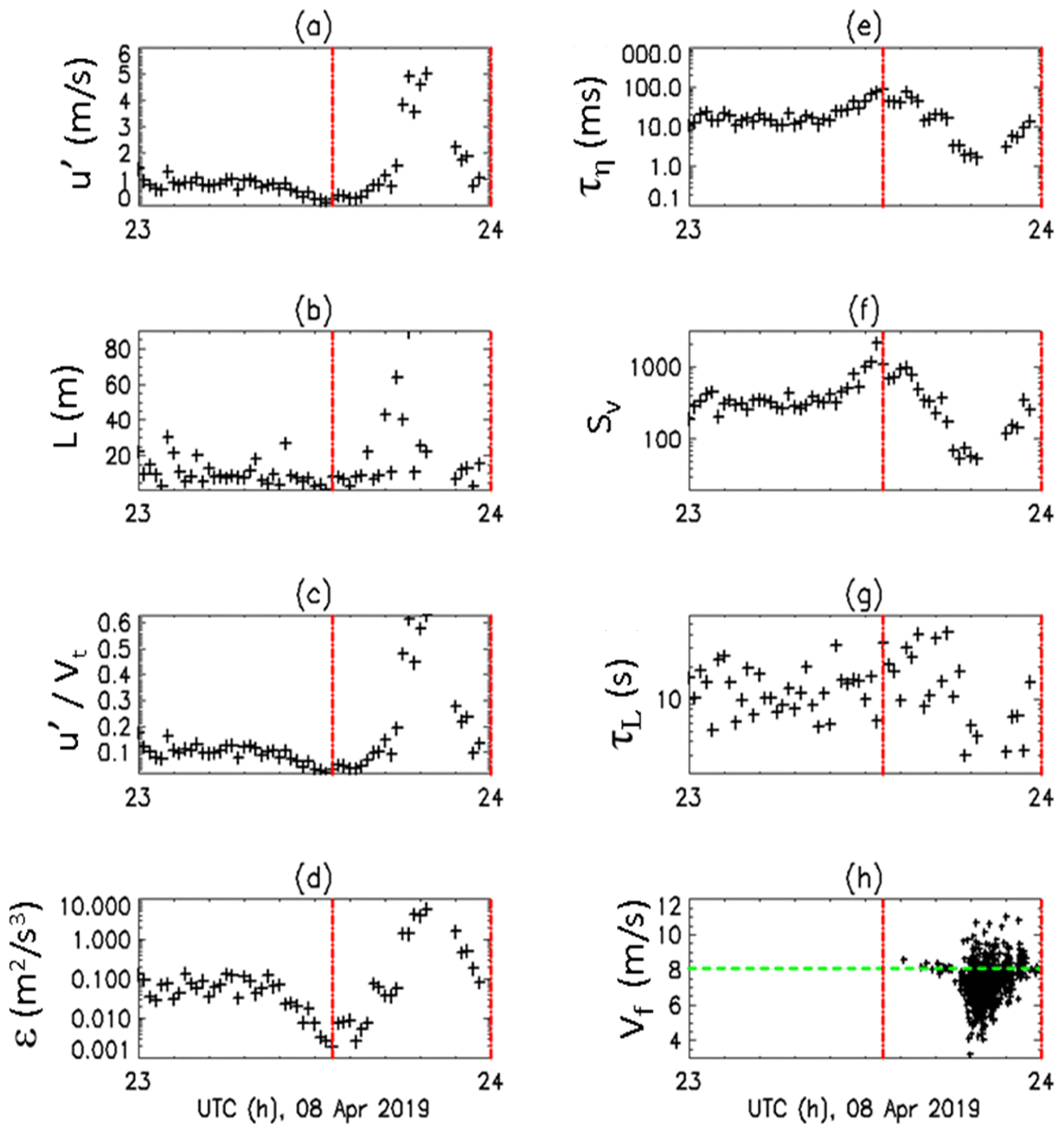
Figure 4(a) to (g) show the pertinent quantities derived from the CSAT-3B 100 Hz horizontal wind data (see text and Table 1 for details) for the 8 April 2020 event from 23:00 to 24:00 UTC; (h) measured fall speeds for the 3 mm drops from 2DVD-SN16 (black) and the expected fall velocity as green line. The two dashed red lines in all panels represent the time interval of rain.
The dissipation rate (ε in Fig. 4d) reaches a maximum of 9 m2 s−3 at 23:45 UTC and <0.01 at 23:30 UTC. The shape (time profile) appears to be symmetric with respect to the time of occurrence of the largest number of 3 mm drops at 23:45 UTC. The shape is highly correlated with shape of the turbulent intensity and the rms velocity fluctuations (u′) in Fig. 4a. The large scale Settling parameter in Fig. 4f reaches a minimum of 80 at 23:45 UTC and its shape is anti-correlated with ε. From the theory and numerical calculations in Fornari et al. (2016), when Sv>1 then gravity dominates the settling behaviour of heavy particles falling in the turbulent flow leading to reduction of the mean fall (settling) velocity relative to the terminal velocity in still air with the fractional reduction depending on the turbulent intensity () as well as the Re. For 2 (3 mm) drop diameters the corresponding Re is 800 (1600) using the terminal velocity. Hence, for a given turbulent intensity () the reduction in the mean settling velocity (relative to terminal) decreases as the Re decreases and in the limit of Stokes regime the settling velocity equals the terminal velocity under still conditions. Stout et al. (1995) explain the mechanism as follows. The smaller drops tend to be disturbed by the eddies and in the limit of, (for example) very low density snow they become (quasi) tracers of the turbulent flow eddies. The heavier drops tend to fall straight down, side stepping the eddies but not completely. These larger heavier drops thus experience a horizontal drag force which depends on relative velocity of the drop with respect to the turbulent flow. This relative velocity is larger for the bigger drops compared to the smaller ones. The horizontal drag force is actually square of the relative velocity between drop and fluid. This non-linear drag force has a vertical component which “slows” down on average the drop settling speed. Now this non-linear drag is present even in non-turbulent flows but there is an enhancement in turbulent flow which goes as (Fornari et al., 2016).
Figure 5a shows another example of a rain event (08:00-09:00 UTC on 9 April 2020) where the fall speeds of the 3 mm drops on average are close to the terminal fall speed shown by the black dashed line. Also shown is the rms velocity fluctuation (u′) which reaches 0 at 08:30 UTC and is <1 m s−1 during the period 08:15–08:45 UTC where the number of 3 mm drops is maximized. The turbulent intensity () is <0.12 which is too small to cause sub-terminal fall speeds. On the other hand, another example from 23 April 2020 is shown in Fig. 5b where three periods centred at (i) 07:30 UTC, (ii) 10:00 UTC and (iii) 20:00 UTC have sufficient numbers of 3 mm drops with, respectively, (i) mean fall speed close to terminal (and turbulent intensity < 0.12), (ii) sub-terminal fall speeds (and intensity around 0.35) and (iii) fall speeds lower than terminal (intensity around 0.25). These results support the theory that larger values of turbulent intensity result in reduced mean fall speeds relative to Vt.
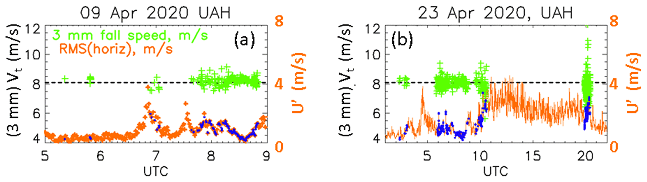
Figure 5(a, b) RMS of horizontal wind speed from the 100 Hz CSAT-3B data (in orange) and 3 mm drop fall speed measurements from 2DVD:SN16 (in green) for the events on 9 April 2020 (a) and 23 April 2020 (b). The blue points are the interpolated rms values corresponding to the timestamps of the 3 mm drops. The black dashed line represents the expected fall speed for the 3 mm drops.
In order to evaluate the statistics of the 2 and 3 mm drop fall speed distributions, data from all six rain events were obtained along with u′. The histograms of the fall speeds were computed for various intervals of the turbulent intensity from to as depicted in the legend of Fig. 6. The shape of the histograms for the different intensity intervals are remarkably symmetric about the mean (or mode) and appear to be Gaussian-like so they are fitted with a Gaussian model shape. The three important points are, (i) the mean fall speed decreases with increasing turbulent intensity, (ii) the standard deviation (or dispersion) increases, and (iii) the effects are larger for the 3 mm sized drops than for the 2 mm drops. Stout et al. (1995) predicted that the reduction in settling speed will increase as the Re increases for a given turbulent intensity, but they did not predict the increase in the dispersion.
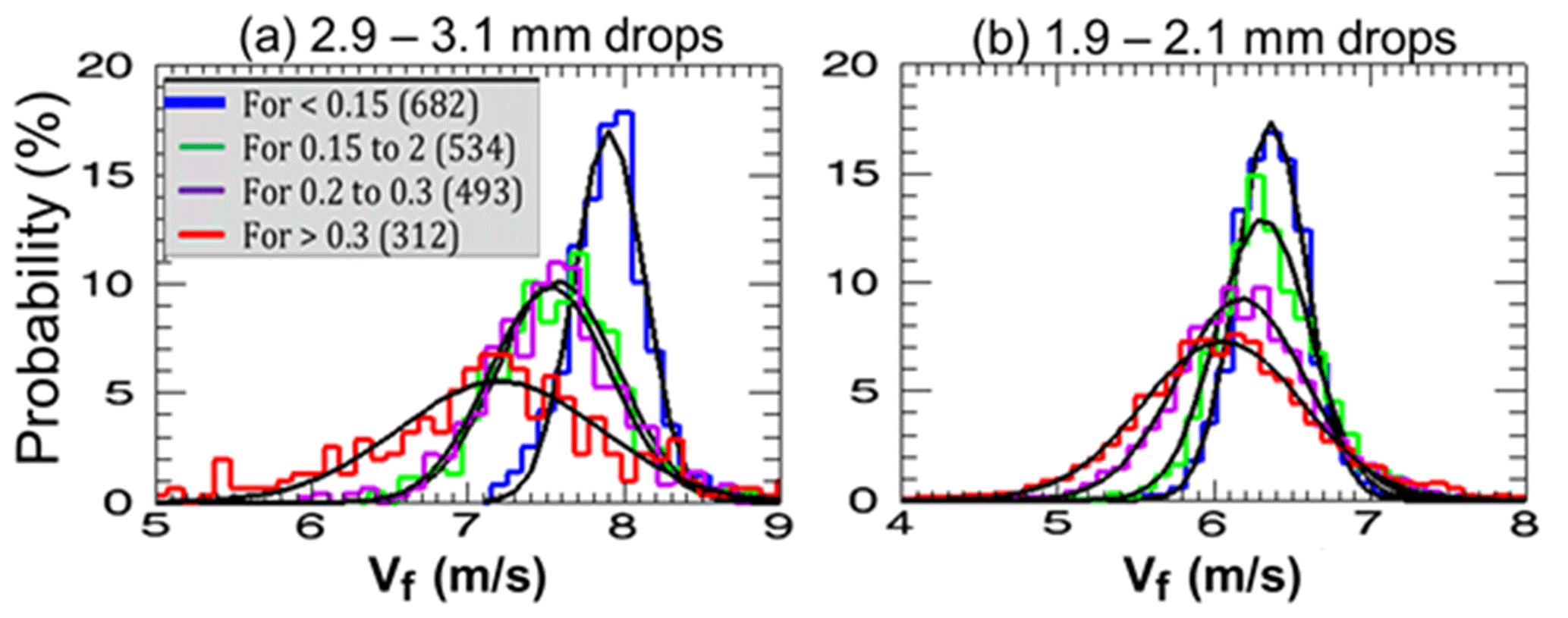
Figure 6Histograms of 3 and 2 mm fall velocities for various intervals of from the six events. Their fitted Gaussian curves (in black) are superimposed.

Figure 7(a) The mean fall speed () versus turbulent intensity for the 2 and 3 mm drops, (b) the deviation of the mean fall speed from the terminal velocity () normalized by Vt and, (c) the standard deviation (σf) versus u′.
Figure 7a shows the mean fall speed () versus turbulent intensity for the 2 and 3 mm drops, Fig. 7b the deviation of the mean fall speed from the terminal velocity () normalized by Vt and Fig. 7c the standard deviation (σf) versus u′. The relative deviation () increases approximately linearly with with a maximum “slowing” down of 10 % for the 3 mm and 6.25 % for the 2 mm for the dataset we have analysed. On the other hand, the σf versus (un-normalized) u′ for both drop sizes are closer to each other (compared to in Fig. 7a) and increase nearly linearly for m s−1. The latter two points are consistent with Fornari et al. (2016) who used direct numerical simulation (DNS) for heavy rigid spheres in turbulent flow. They state that “… although the effect of the turbulence on the mean settling speed depends on , the fluctuations of the settling speed depend mostly on the properties of the turbulent flow (i.e. on u′)”. By fluctuations of the settling speed they mean σf depends weakly on drop size and more on rms velocity fluctuations (u′) whereas the depends on the turbulent intensity (), which clearly is size dependent (Fig. 7a). Fornari et al. (2016) also obtained of around 10 % for in the range 0.2 to 0.3 but they did not model the turbulent scales reflective of atmospheric turbulence.
For completeness, we have estimated the possible effect of finite bin width of 0.2 mm for (2.9–3.1 mm) and (1.9–2.1 mm) sizes on both the relative deviation () and the fractional standard deviation (). Assuming D is uniformly distributed in the bin interval and using the exponential form for fall speed versus D from Atlas et al. (1973), the relative deviation due to finite bin width is very small (<0.03 %) while the fractional standard deviation due to finite bin width is 1.6 % for 2 mm and 0.7 % for 3 mm sizes which are also small.
The other recent DNS (Ren et al., 2020) of mm-sized drop dynamics in turbulent flow showed that % for 3 mm size and 4 % for 2 mm for . Their numerical inlet turbulence generator fixed the turbulence length scale at 0.5 D or 1.5 mm implying that the eddies are of the same scale as D. They show that the mechanism of the mean fall speed “slowing” down in turbulent flow is correlated with a higher drag coefficient, a more complex wake flow with shortened recirculation extent and higher frequency of vortex shedding relative to quiescent flow. However, their DNS does not predict the fall speed dispersion of the magnitude seen in our observations.
The observations of the fall (settling) speeds of 2 and 3 mm sized raindrops with 2D-video disdrometer made simultaneously with wind measurements using a research-grade 3D-sonic anemometer (100 Hz sampling frequency) enabled the acquisition of a unique dataset. Six events recorded are analysed and presented in these Letters. The turbulent intensity, eddy dissipation rate and the integral and Kolmogorov scales were obtained invoking the inertial-dissipation method (Kaimal and Finnigan, 1994) under the assumption of homogeneous isotropic turbulence. The raindrops are obviously heavy inertial particles subjected to gravitational sedimentation in the turbulent atmospheric surface layer. In agreement with prior theoretical, numerical and related experimental studies of similar phenomena we find that the mean fall speed reduces with increasing turbulent intensity nearly linearly, while the fall speed distribution broadens in stronger turbulence. One caveat is whether surface measurements of turbulence are representative of the turbulence in the column of a rainshaft. This can only be tested with a collocated vertical pointing radar (see, Fitch et al., 2021; Garrett and Yuter, 2014). Quantitative comparison of the results obtained herein with prior work has proven elusive due to difficulties in direct numerical simulation of the scales of turbulence in the real atmosphere. Qualitative comparisons have been shown to be in reasonable agreement on the mean fall speed deviation from terminal velocity but the increase in spectral width of the distribution and its Gaussian-like symmetric shape while not unexpected appears as a strong signature in our data. The description of a statistical fall speed pdf (Vf) conditioned on D and turbulent intensity for mm-sized raindrops as opposed to the deterministic Vf versus D relation from Gunn–Kinzer seems appropriate.
The 2DVD data as well as data from the 100 Hz sonic anemometer can be made available via email request to any of the authors: merhala@colostate.edu, bringi@colostate.edu, patrick.gatlin@nasa.gov, matthew.t.wingo@nasa.gov.
MT and VNB were responsible for methodology and data analyses. MW and PNG were responsible for the experimental set-up as well as data curation. Preparation of the original draft was done by VNB and MT. Final review and editing was undertaken by all authors.
The authors declare that they have no conflict of interest.
This article is part of the special issue “Applied Meteorology and Climatology Proceedings 2020: contributions in the pandemic year”.
We wish to thank Karan Venayagamoorthy, Civil and Environmental Engineering Department, Colorado State University, for useful discussions.
This research has been supported by the National Science Foundation, Directorate for Geosciences (grant no. AGS-1901585).
This paper was edited by Fred C. Bosveld and reviewed by two anonymous referees.
Atlas, D., Srivastava, R. C., and Sekhon, R. S.: Doppler radar characteristics of precipitation at vertical incidence, Rev. Geophys. Space Phys., 2, 1–35, 1973.
Beard, K. V.: Terminal velocity and shape of cloud and precipitation drops aloft, J. Atmos. Sci., 33, 851–864, https://doi.org/10.1175/1520-0469(1976)033<0851:TVASOC>2.0.CO;2, 1976.
Bringi, V. N., Thurai, M., and Baumgardner, D.: Raindrop fall velocities from an optical array probe and 2-D video disdrometer, Atmos. Meas. Tech., 11, 1377–1384, https://doi.org/10.5194/amt-11-1377-2018, 2018.
Fitch, K. E., Hang, C., Talaei, A., and Garrett, T. J.: Arctic observations and numerical simulations of surface wind effects on Multi-Angle Snowflake Camera measurements, Atmos. Meas. Tech., 14, 1127–1142, https://doi.org/10.5194/amt-14-1127-2021, 2021.
Fornari, W., Picano, F., Sardina, G., and Brandt, L.: Reduced particle settling speed in turbulence, J. Fluid Mech., 808, 153–167, https://doi.org/10.1017/jfm.2016.648, 2016.
Garrett, T. J. and Yuter, S. E.: Observed influence of riming, temperature, and turbulence on the fallspeed of solid precipitation, Geophys. Res. Let., 41, 6515–6522, 2014.
Good, G. H., Ireland, P. J., Bewley, G. P., Bodenschatz, E., Collins, L. R., and Warhaft, Z.: Settling regimes of inertial particles in isotropic turbulence, J. Fluid Mech., 759, R3, https://doi.org/10.1017/jfm.2014.602, 2014.
Grachev, A. A., Andreas, E. L., Fairall, C. W., Guest, P. S., and Persson, P. O. G.: The Critical Richardson Number and Limits of Applicability of Local Similarity Theory in the Stable Boundary Layer, Bound.-Lay. Meteorol., 147, 51–82, 2013.
Gunn, R. and Kinzer, G. D.: The terminal velocity of fall for water droplets in stagnant air, J. Meteorol., 6, 243–248, https://doi.org/10.1175/1520-0469(1949)006<0243:TTVOFF>2.0.CO;2, 1949.
Kaimal, J. C. and Finnigan, J. J.: Atmospheric boundary layer flows: their structure and measurement, Oxford University Press, New York, 289 pp., 1994.
Larsen, M. L., Kostinski, A. B., and Jameson, A. R.: Further evidence for super terminal drops, Geophys. Res. Lett., 41, 6914–6918, https://doi.org/10.1002/2014GL061397, 2014.
McFarquhar, G.: The effect of raindrop clustering on collision-induced break-up of raindrops, Q. J. Roy. Meteorol. Soc., 130, 2169–2190, 2004.
Montero-Martinez, G. and Garcia-Garcia, F.: On the behavior of raindrop fall speed due to wind, Q. J. Roy. Meteorol. Soc., 142, 2794, https://doi.org/10.1002/qj.2794, 2016.
Montero-Martinez, G., Kostinski, A. B., Shaw, R. A., and Garcia-Garcia, F.: Do all raindrops fall at terminal speed?, Geophys. Res. Lett., 36, L11818, https://doi.org/10.1029/2008GL037111, 2009.
Morrison, H. and Grabowski, W.: Comparison of Bulk and Bin Warm-Rain Microphysics Models Using a Kinematic Framework, J. Atmos. Sci., 64, 2839–2861, 2006.
Nemes, A., Dasari, T., Hong, J., Guala, M., and Coletti, F.: Snowflakes in the atmospheric surface layer: observation of particle–turbulence dynamics, J. Fluid Mech., 814, 592–613, 2017.
Rasmussen, R., Baker, B., Kochendorfer, J., Meyers, T., Landolt, S., Fischer, A. P., Black, J., Thériault, J. M., Kucera, P., Gochis, D., Smith, C., Nitu, R., Hall, M., Ikeda, K., and Gutmann, E.: How well are we measuring snow: the NOAA/FAA/NCAR winter precipitation test bed, B. Am. Meteorol. Soc., 93, 811–829, https://doi.org/10.1175/BAMS-D-11-00052.1, 2012.
Ren, W., Reutzsch, J., and Weigand, B.: Direct Numerical Simulation of Water Droplets in Turbulent Flow, Fluids, 5, 158, https://doi.org/10.3390/fluids5030158, 2020.
Schönhuber, M., Lammer, G., and Randeu, W. L.: One decade of imaging precipitation measurement by 2D-video-distrometer, Adv. Geosci., 10, 85–90, https://doi.org/10.5194/adgeo-10-85-2007, 2007.
Schönhuber, M., Lammar, G., and Randeu, W. L.: The 2-D-videodistrometer, in: Precipitation: Advances in Measurement, Estimation and Prediction, edited by: Michaelides, S. C., Springer, Berlin, Heidelberg, Germany, 3–31, 2008.
Stout, J. E., Arya, S. P., and Genikhovich, E. L.: The effect of nonlinear drag on the motion and settling velocity of heavy particles, J. Atmos. Sci., 52, 3836–3848, https://doi.org/10.1175/1520-0469(1995)052<3836:TEONDO>2.0.CO;2, 1995.
Szakáll, M., Mitra, S. K., Diehl, K., and Borrmann, S.: Shapes and oscillations of falling raindrops – A review, Atmos. Res., 97, 416–425, https://doi.org/10.1016/j.atmosres.2010.03.024, 2010.
Thériault, J. M., Rasmussen, R., Petro, E., Trépanier, J., Colli, M., and Lanza, L. G.: Impact of Wind Direction, Wind Speed, and Particle Characteristics on the Collection Efficiency of the Double Fence Intercomparison Reference, J. Appl. Meteorol. Clim., 54, 1918–1930, 2015.
Thurai, M., Bringi, V. N., Petersen, W. A., and Gatlin, P. N.: Drop shapes and fall speeds in rain: Two contrasting examples, J. Appl. Meteorol. Clim., 52, 2567–2581, https://doi.org/10.1175/JAMC-D-12-085.1, 2013.
Thurai, M., Schönhuber, M., Lammer, G., and Bringi, V.: Raindrop shapes and fall velocities in “turbulent times”, Adv. Sci. Res., 16, 95–101, https://doi.org/10.5194/asr-16-95-2019, 2019.
Wang, L. and Maxey, M.: Settling velocity and concentration distribution of heavy particles in homogeneous isotropic turbulence, J. Fluid Mech., 256, 27–68, https://doi.org/10.1017/S0022112093002708, 1993.
Williams, C. R. and Gage, K. S.: Raindrop size distribution variability estimated using ensemble statistics, Ann. Geophys., 27, 555–567, https://doi.org/10.5194/angeo-27-555-2009, 2009.
Yu, C.-K., Hsieh, P.-R., Yuter, S. E., Cheng, L.-W., Tsai, C.-L., Lin, C.-Y., and Chen, Y.: Measuring droplet fall speed with a high-speed camera: indoor accuracy and potential outdoor applications, Atmos. Meas. Tech., 9, 1755–1766, https://doi.org/10.5194/amt-9-1755-2016, 2016.
Zhang, R., Huang, J., Wang, X., Zhang, J., and Huang, F.: Effects of Precipitation on Sonic Anemometer Measurements of Turbulent Fluxes in the Atmospheric Surface Layer, J. Ocean Univ. China, 15, 389–398, https://doi.org/10.1007/s11802-016-2804-4, 2016.