 | 22 Apr 2021
How to visualize the Urban Heat Island in Gridded Datasets?
Jan D. Keller
The Urban Heat Island (UHI) describes the increase of near surface temperatures within an urban area compared to its rural surrounding. While the concept of the UHI is in itself quite simple, it is more complex to apply it to gridded datasets. The main complication lies in the rural baseline definition. Therefore, we propose three approaches to calculate the spatial UHI representation for gridded datasets from (i) a single point baseline, (ii) an area averaged baseline, and (iii) a nearest neighbor-based baseline field. Based on these approaches, seven methods are tested as an example for a case study utilizing model simulations for three metropolitan areas in Central and Western Europe (Berlin, Paris and Rhine-Ruhr Metropolitan Area). The results show that all methods perform reasonable in absence of complex terrain, biases and large scale temperature gradients. However, with at least one of these features present, the UHI visualization is less prominent or nonexistent, except for the nearest-neighbor approach which consistently shows reasonable spatial characteristics of the UHI across all scenarios.
- Article
(7695 KB) - Full-text XML
- BibTeX
- EndNote


The Urban Heat Island (UHI) is a well-known phenomenon, which has first been described by Howard (1833) and has later been conceptualized (e.g., Oke, 1969). It represents the near-surface characteristic of generally higher temperatures in urban areas compared to cooler temperatures over the surrounding rural areas. This effect originates from the differences in surface types between urban and rural areas which directly affect the energy balance.
The proposed concept was later formalized by Oke (1982) into a theoretical framework for the UHI. Over the last decades multiple studies have confirmed it and found evidence for UHIs in numerous cities around the world (e.g., Yue et al., 2019; Schwarz et al., 2011; Santamouris, 2015) despite the distinct characteristics such as shape or size which vary from city to city. A main effect of the UHI is the increased heat stress and discomfort for humans living or working in urban environments. These characteristics are becoming more and more important with the progressing urbanization and the effect of climate change on the UHI (e.g., Scott et al., 2018; Oleson, 2012).
While the UHI has an impact on various parameters in the boundary layer, most studies focus on near-surface (e.g., 2 m) temperature anomalies following Oke (1982). While the approach is straight forward for station data, it becomes more complex to find a suitable method to calculate and visualize the UHI for gridded data, e.g., satellite observations, model data. Here, we show that the key is to choose an appropriate rural baseline corresponding to the urban area in consideration.
In this paper, we present seven methods to derive the baseline temperatures to determine the spatial UHI structure. We apply the methods to case study simulations of the June 2019 heat wave in Central Europe. Results will be shown and discussed for he metropolitan regions of Berlin, Rhine-Ruhr (both Germany) and Paris (France).
As previously introduced, the methods for visualizing UHI presented in this paper are applied to model data from the June 2019 heat wave over Central Europe (Vautard et al., 2020). During this period, clear sky and stable conditions, which allow for the formation and detection of the UHI (e.g., Arnfield, 2003; Koomen and Diogo, 2017; Li et al., 2020), lasted for over a week.
The corresponding model data comes from simulations with the ICOsahedral Nonhydrostatic Model (ICON) of the German Meteorological Service (Deutscher Wetterdienst, DWD). ICON is the current operational model at DWD for various scales, e.g., global at 13 km or European continent at 6.5 km (ICON-EU). Here, we employ the model in the Limited Area Mode (ICON-LAM) at the operational 2.1 km resolution (D2.1 hereafter) for a Central European domain. For more information about the model structure and schemes, refer to Zängl et al. (2015).
The data visualized here are from a free downscaling simulations of D2.1 forced at the lateral boundary by analyses of the European ICON-EU nest. We take three metropolitan areas as examples, namely Berlin, Paris and the Rhine-Ruhr Metropolitan Area (RRMA) which is the largest German metropolitan area with approximately 11 million inhabitants.
Berlin and Paris have well-defined boundaries of the urban core and more or less circular shapes. The Paris metropolitan area includes several cities and is about 40 to 60 km in diameter, the Berlin metropolitan area incorporates just one other city (Potsdam) and is smaller at a diameter of 25 to 45 km. RRMA includes 13 interconnected cities including Cologne, Essen, Düsseldorf and Bonn and has an irregular shape with a 100 km North-South axis along the river Rhine and an East-West axis in the northern part of about 75 km length.
The UHI is generally defined as the (near surface) temperature difference between an urban area and a neighboring rural area. For point-based observations, the UHI is calculated as the difference between a station in the urban core and a station in the surrounding rural environment. This approach, i.e., the difference between two points, can also be transferred to grid-based data sets such as NWP model output. However, it neglects the added spatial information included in the gridded data and therefore the spatial structure of the UHI itself.
Here, we propose three approaches based on the classic definition of the UHI as described above, but tailored for gridded data sets, e.g., satellite-based observations or model output. These approaches allow for different levels of complexity especially in defining the rural baseline temperature, since for model output the choice of rural and urban points is not limited to the availability of weather stations.
In this case, we define urban and rural gird points by employing a threshold of percentage of the respective land use as provided by a fractional land use data set (e.g., model tiling). For our analysis, we define the threshold for a rural grid point to have an urban land use fraction below 0.2 and an urban grid point with an urban land use fraction above 0.5. In our approaches, the rural baseline is defined by (1) using a single point, (2) a spatial averaged value and (3) a separate nearest neighbor estimate for each grid point.
3.1 Approach 1: Single point
In this approach, the baseline for the UHI calculation is given by a single point value, similar to what is done for station-based UHIs. We identified two possible baselines:
-
M1. The baseline taken from an observation of a rural station.
-
M2. The baseline taken from an arbitrary rural grid point.
It should be noted that method M1 might cause issues with consistency in case of (model) biases or representativity errors. The latter problem can also occur in M2, as the choice of the sample point is arbitrary. Therefore, we choose the value of the grid point with the highest rural land use fraction and a similar elevation (±20 %) to the urban area on average.
3.2 Approach 2: Spatial average
To overcome the limitation of choosing only a single point as reference, the rural baseline can also be obtained as a spatial average over rural grid points. The main step is to define the rural area extension for the averaging process. In general, the included grid points should not be too far away from the urban core to ensure that they are subject to the same atmospheric regime. We define the following four methods for choosing the rural grid point extent:
-
M3. This is the most straight-forward approach and it consists in averaging all rural points in the (arbitrarily chosen) region. The rural grid points should have a low percentage of urban land use, which we set to 0.2 here. However, rural points close to the urban area can still be affected by the UHI therefore polluting the UHI signal.
-
M4. In order to obtain a “clean” rural UHI baseline, we define an subregion (here, using a rectangle) around the urban core and exclude rural points from this area in the averaging.
-
M5. Should the urban area be embedded in complex topography, grid point height has to be taken into consideration to ensures a comparison between similar 2 m temperatures. One way to address this issue is to exclude grid points that have an elevation different from that of the urban core. Here, we exclude those grid points from the M4 subset of rural grid points with an altitude difference of ±20 % from the average elevation of the urban core.
-
M6. Another possibility to address the issue of complex topography is to perform a height-based correction on the temperature field (similar to Sheridan et al., 2010). The reference value used for the correction is the average height of the urban core. We can than calculate the baseline from the same rural grid points as chosen in M4.
A limitation of M6 is related to the height-based correction choice, which is strongly affected by boundary layer stability. Depending on the availability of gridded data to the user, a derived lapse-rate from the full field could be employed. However, this approach requires more input data than surface temperature, elevation and maps of land use. In order to provide a simple straight-forward technique, we therefore choose a standard atmosphere temperature gradient to perform the correction. However, we are aware that this might be inaccurate especially for UHI nighttime conditions.
Although providing a more generalized approach to determine the UHI baseline, spatial averaging still exhibits limitations. The most important are the shape and extent of the rural and urban areas, which can have significant impacts on the results. Here, we choose a rectangular shape for simplicity. However, most cities have complex spatial structures that are difficult to encompass with a simple polygon.
Furthermore, the spatial baseline approach still uses a single value for the whole region which might not be appropriate for points being far apart albeit residing within the urban agglomeration, or in cases of strong horizontal temperature gradients (as later observed in our example for Paris).
3.3 Approach 3: Nearest neighbor
In order to address the limitations of the previous methods, we employ a nearest neighbor approach to define the urban core and to calculate a separate baseline value for each grid point, i.e., to estimate a two-dimensional baseline field.
First, we use an iterative approach to more realistically estimate the spatial structure of the urban core. Therefore, we define a small number of cells inside the urban core as initial seeds. From these, we iteratively determine the respective grid points within a maximum distance of 10 km (i.e., urban interconnection distance) with an urban land use fraction above 0.8. This procedure is then repeated until no new points are added. With the obtained urban core structure, we apply an approach to define a spatially varying rural baseline temperature:
-
M7. This nearest neighbor approach estimates a separate (rural) baseline temperature for each grid point. Specifically, for each grid point we calculate the average temperature of the nearest five rural grid points with an urban land use fraction below 0.2 and a minimal distance of 8 km to the determined main urban core. The UHI field is then obtained by subtracting the 2 m temperature field from the baseline field. In our implementation, the ball tree method (e.g., Friedman et al., 1977) allows for finding the nearest neighbors for each grid point at low computational cost.
The resulting representations of the UHI are compared in the following section.
The previously presented methods are now applied to the 2 m temperature field of the aforementioned metropolitan agglomerations Berlin, Paris and Rhine-Ruhr metropolitan area at 22:00 UTC on 25 June 2019 as provided by the ICON model output (see Sect. 2). The chosen date corresponds to the peak of the June 2019 heatwave over Central Europe.
4.1 Baseline
Figure 1 illustrates the grid points chosen for the calculation of the rural baseline temperature for the three regions.
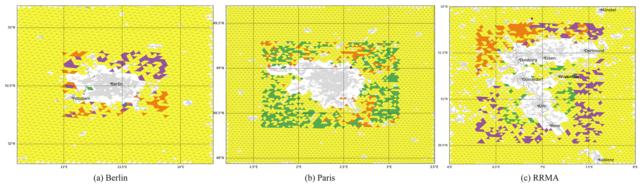
Figure 1Color-coded grid point selection for all 7 methods for Berlin, Paris and the Rhine-Ruhr Metropolitan Area (a–c). Triangles represent the model grid-point, while the red circle is the station used. The GlobCover original 1 km resolution urban land use data is shown in light-grey shading as reference.
The station location used in M1 is shown as a red dot in each area, the grid cell used as reference in M2 as a blue triangle. Most of the other methods at least in part rely on the same subset of grid points. M3 includes all the purple, orange and green grid points, the latter being the ones exclusive to this method. M4 and M6 are based on the same selection which includes the orange- and purple-colored cells while M5 only uses the orange triangles. The nearest neighbor approach M7 uses for each grid point the nearest five cells from all yellow, purple, orange and blue triangles as well as most of the green ones.
4.2 Urban Heat Island representation
This section presents and discusses the UHI representations with respect to the baselines as derived from the methods M1 to M7 for the case study. The case study is only intended as an example and we will not go into detail about physical processes involved in the phenomenon.
As expected, the various methods lead to (in part significant) differences in the baseline temperature. The obtained values (expressed in Celsius) are summarized in Table 1.
Table 1Case study baseline values (in Celsius) for UHI calculation. Values for M7 have been averaged on the M4 area as comparison.
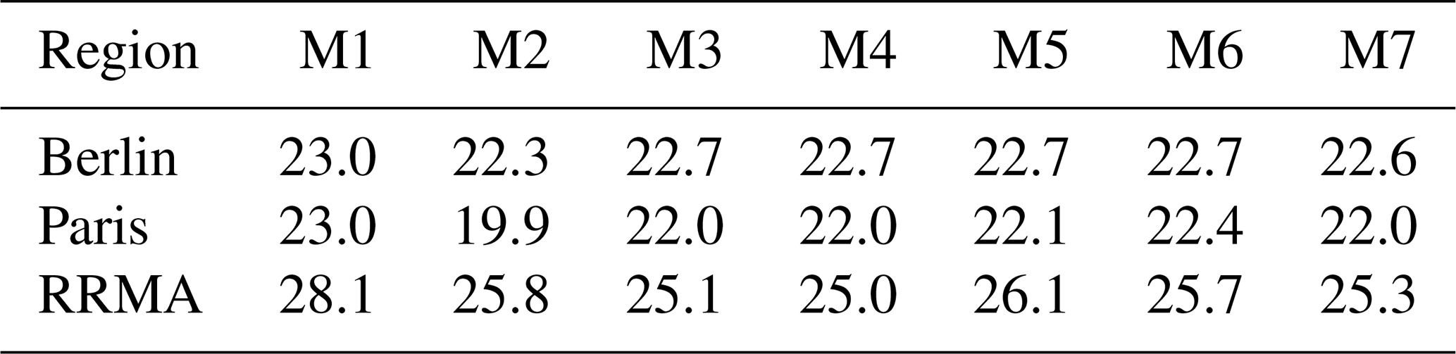
Since M7 has not a constant baseline value, we take the average of the M7 baseline field over all grid points used in M4 for comparison.
In general, there are distinct temperature differences between the regions as the heat wave on 25 June was stronger over the western part of Germany compared to eastern Germany and northern France. This can basically be seen in the M1 baseline temperatures which originate from the respective station measurements. Berlin shows a low variability (<1 ∘C) among the various baseline values for the seven methods, with the largest difference between the two single point selections M1 and M2. A similar behavior is observed for the Paris baseline values. RRMA shows a higher variability with differences of more than 2 ∘C between some of the methods.
The impact of the different baseline methods on the horizontal UHI representation in the model data is discussed in the following. The M1-derived UHI is shown for the three regions in Fig. 2. As the method is based on observational data, it is clear that the model exhibits a strong cold bias for RRMA of about −2 ∘C and to a lesser extent over Paris (−1 ∘C).
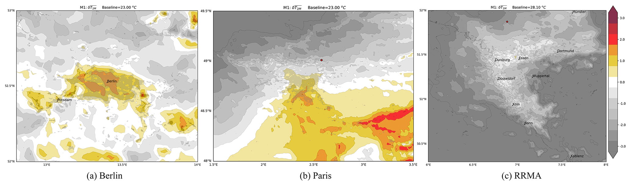
Figure 2UHI calculated with M1 on the original grid (no interpolation) for Berlin, Paris and the Rhine-Ruhr Metropolitan Area (a–c). The location of the weather station used as baseline is shown as a red dot, only when it is in the vicinity of the urban area.
For Berlin, the model does not exhibit a strong bias and a reasonable UHI representation with a magnitude of 1 to 1.75 ∘C. The Paris region exhibits a strong North to South temperature gradient thus masking a potential UHI. Due to the model bias, the RRMA has no positive UHI for M1 albeit the urban core being much warmer than the surrounding rural area.
When using a single-point rural reference from model data (method M2), the biases disappear and the magnitude of the UHI becomes more realistic. As expected, the UHI value for the reference point outside the urban core is zero, i.e., white shading in Fig. 3. For all three regions, the UHI values are higher compared to M1. However, for Berlin the UHI extent is much too large and the gradient is not very sharp whereas the overall temperature gradient in the Paris region makes a potential UHI invisible. For RRMA, method M2 produces a reasonable looking UHI, however, its spatial extent being exaggerated in the northern part. M2 also highlights the complex topography south of the urban core in RRMA.
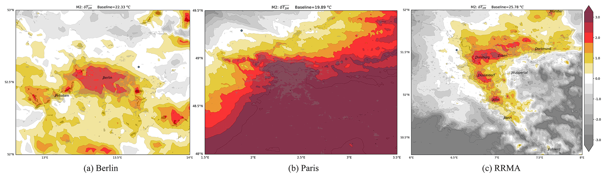
Figure 3UHI calculated with M2 on the original grid (no interpolation) for Berlin, Paris and the Rhine-Ruhr Metropolitan Area (a–c). The location of the grid-point used as baseline is shown here as a blue dot, or in Fig. 1 as a blue grid-point (triangle).
With area-averaging, we try to address the issue of representativity and bias occurring in the single-point approaches. Averaging over all rural grid points in the region (M3) leads to a more balanced baseline temperature around the urban core. The corresponding UHI representations as shown in Fig. 4 indicate that for Berlin and Paris, the spatial pattern becomes more realistic albeit for Paris, the gradient still masks a possible UHI structure in the southern part of the city. For RRMA, the extent of the UHI increases further beyond the boundaries of the urban areas.
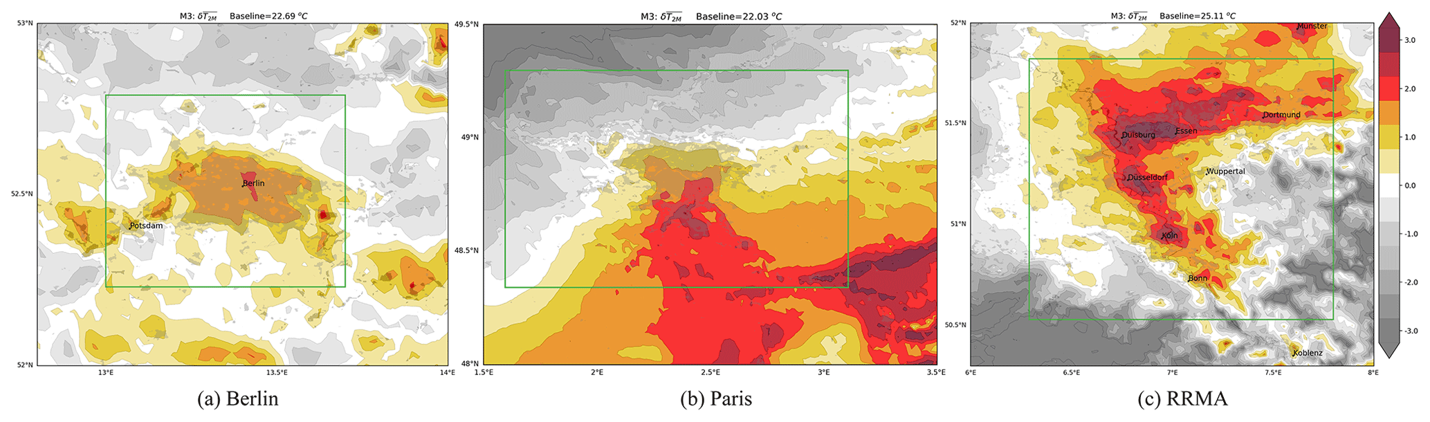
Figure 4UHI calculated with M3 on the original grid (no interpolation) for Berlin, Paris and the Rhine-Ruhr Metropolitan Area (a–c), the limit of the rural points used in the baseline is shown here in the green lines, or in Fig. 1 as the sum of green, purple and orange grid-points.
The results of the other spatial-averaging methods (c.f. Fig. 4 to Figs. A1–A3 in the appendix) are qualitatively very similar as they also only provide one baseline value for each region. Differences for the methods M4 and M5 are mostly only visible for RRMA. The spatial structure and amplitude of M4 is similar to M3 and that of M5 to M2. For the method M6, which employs a simple height-correction to the temperature field, no significant changes can be found for Berlin and Paris. For the latter region, a further exaggeration of UHI in the southeastern part of domain. For RRMA, the results also show some issues in the topographically complex terrain in the southeast of the domain, but the basic structure of the UHI over the metropolitan areas is similar to the other methods.
The basic shortcoming of the aforementioned methods with respect to the spatial representation of the UHI is that only a single value (or constant field) is used as a baseline. Method M7 provides a separate baseline value for each grid point and therefore allows for a more realistic calculation of the UHI. The spatial representation of the baselines for the case study can be found in Fig. B1 in the appendix.
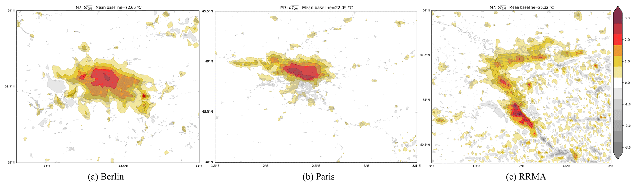
Figure 5UHI as calculated with M7 on the original grid (no interpolation) for Berlin, Paris and the Rhine-Ruhr Metropolitan Area (a–c).
Figure 5 shows the resulting UHI patterns for M7 in the three regions. In general, the negative values mostly disappear with the respective baseline values being close to the actual temperature in non-urban areas. Further, the UHI is mostly restricted to the urban core with its extent for Berlin covering most urban grid points and its peak above 2.25 ∘C. For Paris, the UHI covers the northern half of the metropolitan area as its southern half is not significantly warmer than the surrounding rural areas. Therefore, the UHI representation seems to be realistic for this case. For the RRMA, the UHI is more scattered across all urban agglomerates and with slightly lower peaks (2 ∘C) compared to the other methods. As the employed nearest-neighbour approach uses several grid points to calculate the baseline, spurious positive and negative values might occur in complex topography as can be found in the south-eastern part of the RRMA domain.
The originally proposed UHI calculation using observed urban and rural station temperature data is trivial. However, an increasing number of studies are now employing numerical weather prediction models or satellite-based gridded observations to investigate and analyze the UHI. While the theoretical concept is clearly defined, it is much more complicated to come up with a practical implementation for calculating the for gridded measurements or model data to account for the complex morphology of cities and their surroundings.
In this study, we tested various methods on model data for three urban agglomerations. Straight forward approaches using either a single point (methods M1, M2) or a spatial average (M3 to M6) to determine the baseline can result in reasonable approximations of the UHI (e.g. for the Berlin case in our study) especially for its peak amplitude in the urban core. However, these methods are also prone to biases and under- or overestimation of the UHI extent. These issues arise from how the baseline temperature is estimated as well as the major shortcoming of representing the environment in which the respective urban agglomerate is embedded as a single value.
The often dominating complexity of the interaction between land use, topography and atmospheric dynamics makes a more sophisticated approach necessary. Therefore, we determine a rural baseline temperature for each grid point using a nearest neighbor approach (M7). This allows for the consideration of heterogeneities in and surrounding the urban core such as complex topography or temperature gradients. We find, that the resulting spatial UHI representation for the three case study regions seem realistic given the underlying model resolution. The strengths of method M7 can be seen in the Paris region where a strong meridional temperature gradient makes it impossible to identify a clear UHI for all other methods. Potential artefacts when using M7 which may manifest as spurious UHI values in complex terrain (as can be seen for RRMA) are, however, rather small and can be neglected with respect to the overall benefits of the method.
This appendix contains the figures referred to but not included in Sect. 4. As explained, some UHI methods have been moved to the appendix due to the fact that only minor differences can be observed in the rural baseline values. For completeness, the results are presented for the case studies for methods M4 (Fig. A1), M5 (Fig. A2) and M6 (Fig. A3).
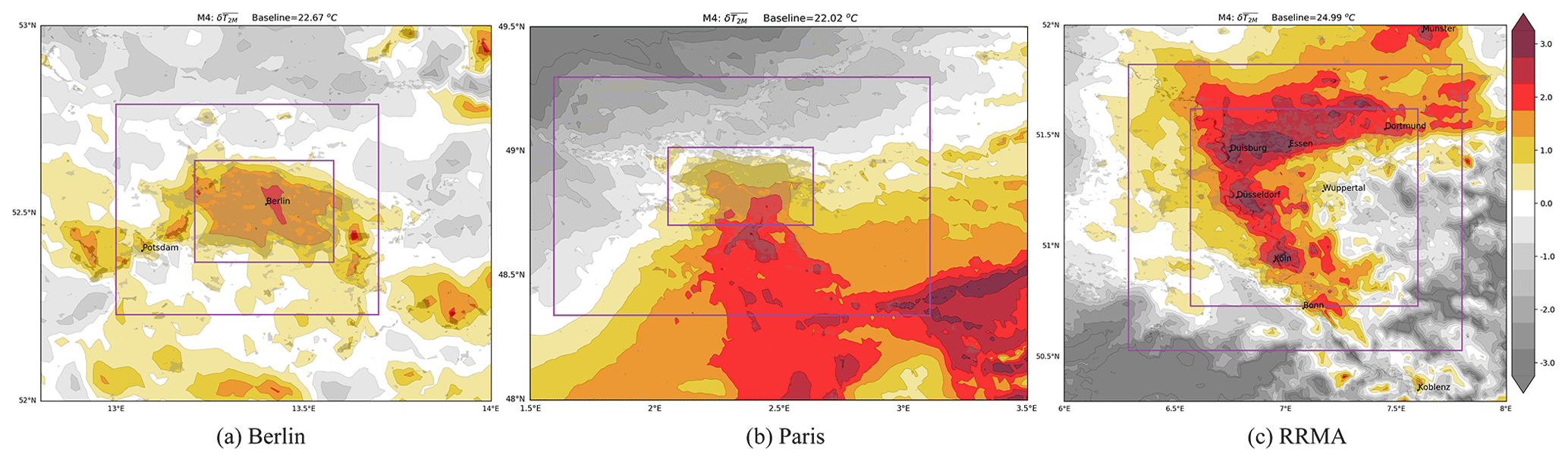
Figure A1UHI calculated with M4 on the original grid (no interpolation) for Berlin, Paris and the Rhine-Ruhr Metropolitan Area (a–c), the rural area used as baseline is encompassed by the two purple rectangles, or in Fig. 1 as the sum of purple and orange grid-points.

Figure A2UHI calculated with M5 on the original grid (no interpolation) for Berlin, Paris and the Rhine-Ruhr Metropolitan Area (a–c), the rural area used as baseline is encompassed by the two orange rectangles, or in Fig. 1 as the orange grid-points.
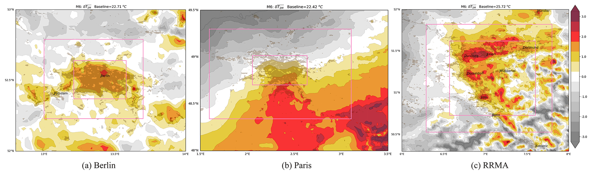
Figure A3UHI calculated with M6 on the original grid (no interpolation) for Berlin, Paris and the Rhine-Ruhr Metropolitan Area (a–c), with the height gradient correction. The baseline used is the same as M4.
This appendix contains Fig. B1 depicting the two-dimensional baseline fields obtained for the case studies with method M7.
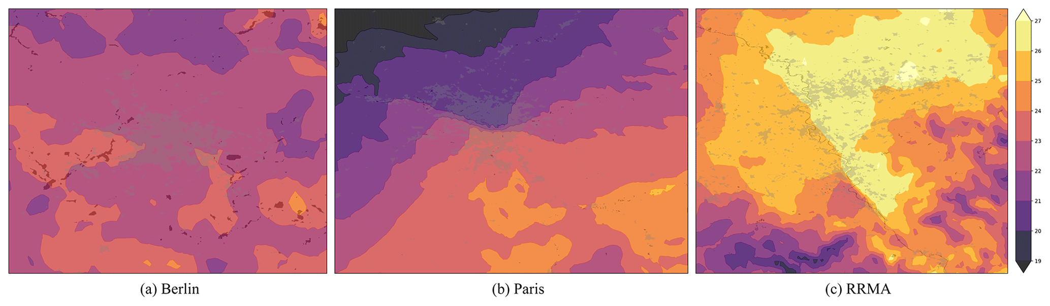
Figure B1Baseline fields as estimated with M7 on the original grid (no interpolation) for Berlin, Paris and the Rhine-Ruhr Metropolitan Area (a–c).
The code is available at: https://doi.org/10.5281/zenodo.4686665 (Valmassoi and Keller, 2021a).
The data is available at: https://doi.org/10.5281/zenodo.4700304 (Valmassoi and Keller, 2021b).
AV and JDK designed the methodology. AV carried out the experiments and implemented the code of the analysis with the support of JDK. AV prepared the manuscript. AV and JDK reviewed it iteratively.
The authors declare that no competing interests are present.
This article is part of the special issue “Applied Meteorology and Climatology Proceedings 2020: contributions in the pandemic year”.
This work has been conducted in the framework of the Hans-Ertel-Centre for Weather Research.
This work has been conducted with funding by the German Federal Ministry for Transportation and Digital Infrastructure (grant no. BMVI/DWD 4818DWDP5A).
This paper was edited by Pavol Nejedlik and reviewed by Radim Tolasz and one anonymous referee.
Arnfield, A. J.: Two decades of urban climate research: A review of turbulence, exchanges of energy and water, and the urban heat island, Int. J. Climatol., 23, 1–26, https://doi.org/10.1002/joc.859, 2003. a
Friedman, J. H., Louis Bentley, J., Ari Finkel, R., and Frmdman, J.: An Algorithm for Finding Best in Logarithmic Expected Time, ACM Transactions on Mathematical Software, 3, 209–226, https://doi.org/10.1145/355744.355745, 1977. a
Howard, L.: The climate of London: deduced from meteorological observations made in the metropolis and at various places around it, Harvey and Darton, J. and A. Arch, Longman, Hatchard, S. Highley and R. Hunter, 3. Edn., Joseph Rickerby, Printer, Sherbourn Lane, London, 1833. a
Koomen, E. and Diogo, V.: Assessing potential future urban heat island patterns following climate scenarios, socio-economic developments and spatial planning strategies, Mitig. Adapt. Strat. Gl., 22, 287–306, https://doi.org/10.1007/s11027-015-9646-z, 2017. a
Li, Y., Schubert, S., Kropp, J. P., and Rybski, D.: On the influence of density and morphology on the Urban Heat Island intensity, Nat. Commun., 11, 2647, https://doi.org/10.1038/s41467-020-16461-9, 2020. a
Oke, T. R.: Towards a more rational understanding of the urban heat island, McGill Climatol. Bull., 5, 1–21, 1969. a
Oke, T. R.: The energetic basis of the urban heat island, Q. J. Roy. Meteor. Soc., 108, 1–24, 1982. a, b
Oleson, K.: Contrasts between Urban and rural climate in CCSM4 CMIP5 climate change scenarios, J. Climate, 25, 1390–1412, https://doi.org/10.1175/JCLI-D-11-00098.1, 2012. a
Santamouris, M.: Analyzing the heat island magnitude and characteristics in one hundred Asian and Australian cities and regions, Sci. Total Environ., 512–513, 582–598, https://doi.org/10.1016/j.scitotenv.2015.01.060, 2015. a
Schwarz, N., Lautenbach, S., and Seppelt, R.: Exploring indicators for quantifying surface urban heat islands of European cities with MODIS land surface temperatures, Remote Sens. Environ., 115, 3175–3186, https://doi.org/10.1016/j.rse.2011.07.003, 2011. a
Scott, A. A., Waugh, D. W., and Zaitchik, B. F.: Reduced Urban Heat Island intensity under warmer conditions, Environ. Res. Lett., 13, 064003, https://doi.org/10.1088/1748-9326/aabd6c, 2018. a
Sheridan, P., Smith, S., Brown, A., and Vosper, S.: A simple height-based correction for temperature downscaling in complex terrain, Meteorol. Appl., 17, 329–339, https://doi.org/10.1002/met.177, 2010. a
Valmassoi, A. and Keller, J. D.: arjanna/UHI-calculation: (Version V1.1), Zenodo [code], https://doi.org/10.5281/zenodo.4686665, 2021a. a
Valmassoi, A. and Keller, J. D.: Data used in “How to visualize the Urban Heat Island in Gridded Datasets?”, Zenodo [data set], https://doi.org/10.5281/zenodo.4700304, 2021b. a
Vautard, R., Van Aalst, M., Boucher, O., Drouin, A., Haustein, K., Kreienkamp, F., Van Oldenborgh, J., Otto, F. E. L., Ribes, A., Robin, Y., Schneider, M., Soubeyroux, J.-M., Stott, P., Seneviratne, S. I., Vogel, M. M., and Wehner, M.: Human contribution to the record-breaking June and July 2019 heat waves in Western Europe, Environ. Res. Lett., 15, 094077, https://doi.org/10.1088/1748-9326/aba3d4, 2020. a
Yue, W., Liu, X., Zhou, Y., and Liu, Y.: Impacts of urban configuration on urban heat island: An empirical study in China mega-cities, Sci. Total Environ., 671, 1036–1046, https://doi.org/10.1016/j.scitotenv.2019.03.421, 2019. a
Zängl, G., Reinert, D., Rípodas, P., and Baldauf, M.: The ICON (ICOsahedral Non-hydrostatic) modelling framework of DWD and MPI-M: Description of the non-hydrostatic dynamical core, Q. J. Roy. Meteor. Soc., 141, 563–579, https://doi.org/10.1002/qj.2378, 2015. a
- Abstract
- Introduction
- Case study data
- UHI calculation
- Results
- Conclusions
- Appendix A: Visualization of the UHI for the other presented methods
- Appendix B: UHI baseline
- Code availability
- Data availability
- Author contributions
- Competing interests
- Special issue statement
- Acknowledgements
- Financial support
- Review statement
- References