 | 11 May 2021
Using machine learning to produce a very high resolution land-cover map for Ireland
Eoin Walsh
Geoffrey Bessardon
Emily Gleeson
Priit Ulmas
Land-cover classifications in the form of maps are required for numerical modelling of weather and climate. Such maps are often of coarse resolution and are infrequently updated. Here we propose a novel approach for land-cover classification using a Convolutional Neural Network machine learning algorithm to segment satellite images into various land-cover classes. Sentinel-2 satellite imagery, the CORINE land-cover database and the BigEarthNet dataset are used. A 10 m resolution map, called the Ulmas-Walsh map, has been created for Ireland that outperforms ECO-SG in terms of accuracy, as well as demonstrating a capacity for identifying features not labelled correctly in CORINE. The map can be updated on demand for any time of the year, subject to cloud cover. This is particularly useful for regions with large seasonal variation in land classifications such as Turloughs – seasonal lakes, flood plains and rotational crops.
- Article
(18547 KB) - Full-text XML
- BibTeX
- EndNote


To accurately model Earth surface processes the Numerical Weather Prediction (NWP) systems used for operational weather forecasting require information on land-cover classifications such as urban areas, the types of nature – trees, crops, grassland etc., water bodies and more. NWP models need this information to compute surface parameters used in turbulent, radiative, heat, and moisture fluxes estimations. Accurate estimations of these fluxes is essential for weather prediction as the surface is where most of the energy and water exchanges happen.
To produce land-cover maps, observations acquired through remote-sensing (sometimes complemented with ground-based observations) are gathered into classes or labels based on features that are identifiable in the observations and that the map producer wants to distinguish. Thus, there is no generic way to make a land-cover map which means that different meteorological organisations use different land-cover descriptions in their models.
The Integrated Forecasting System (IFS) cycle 47r1 (ECMWF, 2020) of the European Centre for Medium-Range Weather Forecasts (ECMWF) and the latest configurations of the UK Met Office Unified Model (UM; Walters et al., 2019) use the Global Land-Cover Characteristics database (GLCC; Loveland et al., 2000). A variation on GLCC is also used by the COSMO (Consortium for Small-Scale Modelling) consortium (Doms et al., 2013) where GLCC is substituted by CORINE (Coordination of Information on the Environment; European Environment Agency, 2017) data where available and the vegetation is evaluated using the Global land-cover 2000 (Bartholomé and Belward, 2005) dataset. Met Éireann, the Irish Meteorological Service, uses the HARMONIE-AROME canonical model configuration (CMC) of the shared ALADIN-HIRLAM NWP system for short-range operational weather forecasting (see Appendix E for more information on HARMONIE-AROME and ALADIN-HIRLAM). The default surface land-cover in HARMONIE-AROME is the ECOCLIMAP (Bengtsson et al., 2017) global land-cover database developed by Météo-France in partnership with the scientific community (Masson et al., 2003; Faroux et al., 2013; CNRM, 2018).
In ECOCLIMAP a cover type is defined as any combination of the following four land-use types, known as “tiles”: sea, inland water (lakes, rivers, …), urban and nature. The nature tile is further divided into 19 classes most of which are vegetation. Note that we will refer to the 19 classes as “vegetation” classes even though three of these contain no vegetation – bare land, rocks and permanent snow i.e. glaciers. Combinations of these vegetation classes form the vegetation covers in ECOCLIMAP-I and ECOCLIMAP-II (Masson et al., 2003; Faroux et al., 2013).
The latest version of ECOCLIMAP, ECOCLIMAP-SG (ECO-SG), was introduced in 2018 and is planned for use in future versions of HARMONIE-AROME. Rather than using the CORINE land cover map as a base map, combined with other datasets (Masson et al., 2003; Faroux et al., 2013), the ECO-SG base map is the ESA-CCI (European Space Agency Climate Change Initiative; European Space Agency, 2017) 2015 land cover map, and CORINE labelling is only used over urban areas (CNRM, 2018). ECO-SG uses pure rather than mixed vegetation classes. This classification reduces the number of land-covers from 478 in ECOCLIMAP-II to 33 in ECO-SG, making ECO-SG classification more straightforward and more suitable for automation in the future. An evaluation of ECO-SG showed an improvement in the representation of water bodies compared to ECOCLIMAP-II (Samuelsson et al., 2020). However, some limitations in the performance of the current HARMONIE-AROME configuration are attributed to surface processes and physiography issues (Bengtsson et al., 2017). The use of local physiographic datasets to identify and correct ECOCLIMAP-II inaccuracies over Iceland led to an improvement in wind forecasts (Petersen et al., 2017) and motivated us to compare the different iterations of ECOCLIMAP against local physiographic datasets for Ireland.
A comparison between the Prime2 land-cover map (Ordnance Survey Ireland, 2014), considered to be Ireland's reference land-cover map (Green, 2015), and ECO-SG suggested that sparse urban areas are underestimated and instead appear as vegetation areas in ECO-SG (Bessardon and Gleeson, 2019). Further analysis showed that grassland tends to be overestimated and appears in place of sparse urban areas and other vegetation covers (Met Éireann internal communication). Thus, further work was needed to assess and improve ECO-SG over Ireland.
In the context of the development of shared operational weather forecasting such as in METCoOp (Meteorological Co-operation and Operational NWP – collaboration between Norway, Sweden, Finland and Estonia) and United Weather Centres (UWC-West is a collaboration between Ireland, Iceland, Denmark and the Netherlands; UWC-East includes METCoOp, Latvia and Lithuania), solutions to improve the accuracy of ECO-SG over Ireland need to be applicable for, or as a minimum should not create issues in, other countries within the operational domain.
Discussions with surface physics specialists raised concerns about the insertion of national observation datasets into a global dataset because doing this could potentially create artificial borders in the dataset which could have implications such as artificial jumps in surface fluxes. For example, in Ireland this could lead to issues in the dataset across the border between the Republic of Ireland and Northern Ireland. Artificial borders formed by the insertion of national data into a global database like ECOCLIMAP would not be ideal from a forecasting point of view. Moreover, Prime2 does not provide information over Irish mountains which cover a substantial part of the country (Cawkwell et al., 2018). Thus, local datasets should be used solely as a reference where available. Future iterations of HARMONIE-AROME will be at a higher resolution and therefore will require higher resolution physiographic inputs. It is thus desirable that improvements in land-cover maps can potentially be of very high resolution. Also, land-cover is not static in time due to human activity and climate change.
A map that can be regularly updated is necessary in order to reflect such changes which can impact on meteorological parameters. Ulmas and Liiv (2020) used a convolutional neural network (CNN) trained with the “BigEarthNet” (Sumbul et al., 2019) dataset to create a land-cover map with CORINE labels using Sentinel-2 satellite imagery (Bertini et al., 2012) over Estonia. This method showed a capability of increasing the accuracy of CORINE. CORINE is considered to be of good accuracy with the two latest iterations (2012, 2018) estimated to be more than 85 % accurate (Jaffrain, 2017; European Environment Agency, 2017) which is superior to the 75.4% estimated accuracy of ESA-CCI 2015, the base map for ECO-SG (European Space Agency, 2017). This method can consequently significantly improve the accuracy of ECO-SG and can produce a land-cover map at Sentinel-2 resolution (10×10 m) which is 900 times higher than that of ECO-SG (300×300 m). The method has the potential to be used for any area covered by Sentinel-2 and offers the possibility of frequent updates to account for seasonal changes in land-cover.
A CNN is a machine learning (ML) algorithm architecture used mainly for computer vision tasks. ML is an area of data science which involves developing algorithms that improve through experience (Mitchell, 1997). The application of ML techniques to the study of weather and climate is rapidly growing (Jones, 2017). For example, ML can help forecasters with the decision-making process (Karstens et al., 2015, 2016). It would be challenging to develop an NWP model purely by training ML algorithms (Dueben and Bauer, 2018). Nevertheless, the performance of ML-based model parametrisations has proven successful and such are used in the parametrization of radiation (Chevallier et al., 2000; Krasnopolsky et al., 2005), ocean physics (Krasnopolsky et al., 2002; Tolman et al., 2005) and convection (Krasnopolsky et al., 2013) for example. The estimation of surface roughness and turbulent fluxes through ML also yielded better performance than physical models (Hu et al., 2020). ML algorithms can be used on NWP model outputs to optimise precipitation forecasts by increasing the representation of rainfall extremes (Krasnopolsky and Lin, 2012), and storm duration (McGovern et al., 2017). The optimisation of ensemble weather forecasts also uses ML (Rasp and Lerch, 2018; Grönquist et al., 2020). A ML visibility diagnostic showed some improvement in visibility forecasting in comparison with an operational visibility diagnostic scheme (Bari and Ouagabi, 2020). ML is also used in microwave radiometry (Jung et al., 1998; Radiometer Physics, 2014) and surface observation quality control (de Vos et al., 2019; Napoly et al., 2018; Båserud et al., 2020).
Some land description inputs produced using ML techniques are already used operationally. For example, ML algorithms trained using national in-situ soil inventories and satellite data were used to produce recent soil maps: the LandUse and Cover Area frame Statistical survey (LUCAS) topsoil (Ballabio et al., 2016), and the SoilGrids (Hengl et al., 2017) datasets. The introduction of ML techniques in soil map generation enabled the production of higher resolution, globally complete, accurate maps (Hengl et al., 2017). Other physiographic inputs such as forest canopy height (Simard et al., 2011; Li et al., 2020) are also developed using ML in association with satellite imagery. While several studies show the benefit of applying ML to satellite imagery for land-cover mapping over Ireland (Nitze et al., 2015; Connolly, 2018; Cawkwell et al., 2018) none of these studies has led to a dataset covering all of Ireland or a comparison being done with ECO-SG. The work presented in this paper led to the production of a very high resolution land-cover map for Ireland following the method of Ulmas and Liiv (2020).
The paper is organised as follows: Sect. 2 introduces the Sentinel-2, CORINE and BigEarthNet datasets used in the generation of the land-cover map for Ireland. Section 3 provides details about the ML approaches used including training the model and the models created. The results are included in Sect. 4 where the resulting map is compared to CORINE and ECO-SG. Finally, Sect. 5 includes the discussion and conclusions.
This section describes the datasets used in this study including information on the pre-processing required. Section 2.1 provides details about the Sentinel-2 satellite imagery used. Section 2.2 describes the CORINE land-cover dataset. Information on the BigEarthNet dataset, consisting of Sentinel satellite imagery appended with land-cover information, is detailed in Sect. 2.3.
2.1 Sentinel-2 satellite data
The Sentinel-2 Earth Observation Satellite (Bertini et al., 2012) gathers data across 13 spectral bands at three spatial resolutions (10, 20 and 60 m). The visible light channels were considered most appropriate as a starting point for researching the use of ML in creating a meteorological land-cover map, as they have been widely use in earth observation ML applications successfully already. We acquired data at 10 m resolution (we opted for the highest resolution available) from bands 2, 3 and 4 which correspond to the blue, green and red bands, which when combined gave a RGB image. The use of other bands has not been ruled out for future developments in this work. The data were acquired via the Copernicus Open Access Hub (https://scihub.copernicus.eu/, last access: 30 April 2021) and are composed of 25 tiles over Ireland (see Fig. 1). Multiple samples of each tile were obtained to minimise significant cloud cover in the final composite image. Each Sentinel-2 tile is 109.8 km2, with an overlap of 4.9 km with neighbouring tiles.
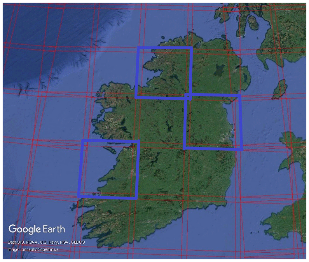
Figure 1Satellite image of Ireland with various Sentinel-2 tiles outlined in red. The tiles highlighted in blue were used to train the ML algorithms (Source: https://www.google.com/earth/, last access: 30 April 2021).
2.2 CORINE land-cover dataset
In order to train a supervised ML algorithm, such as a CNN, the training data requires outputs as well as inputs. In our case, the algorithms were trained to output land-cover map predictions based on Sentinel-2 satellite imagery input data. The CORINE land-cover dataset, hereafter CORINE, most recently updated in 2018 (European Environment Agency, 2017) was used as the training outputs. CORINE was used as the training data output because it is considered to be quite accurate. The 2012 iteration was estimated to be 85 % accurate (Jaffrain, 2017) and the 2018 iteration is thought to be of even higher accuracy (European Environment Agency, 2017).
CORINE has a tiered 3-level labelling system. Level 1 (primary) is the most generic while level 3 (tertiary) is the most detailed. There are 5 labels in level 1, 15 labels in level 2 (secondary) and 44 labels in level 3. Levels 1 and 2 were the focus of this work because it was undertaken as part of a 12-week PhD work placement and was time constrained; extension of the work to tertiary cover types is currently underway in a separate study. The CORINE map is only available in its tertiary label form. These labels were converted to their primary and secondary tier forms for use in our ML algorithms (see https://land.copernicus.eu/user-corner/technical-library/corine-land-cover-nomenclature-guidelines/html/index.html, last access: 30 April 2021, for CORINE labelling hierarchy details).
The resolution of the CORINE dataset is 100×100 m, whereas the Sentinel-2 satellite images have a resolution of 10 m. Each satellite image segment of size 120×120 px corresponds to a CORINE segment of size 12×12 px. The CORINE segments were resized to 120×120 px using nearest-neighbour interpolation so that the CORINE data and the Sentinel-2 data had the same resolution, as the CNN used requires this.
2.3 BigEarthNet
BigEarthNet (Sumbul et al., 2019) is a large scale Sentinel-2 satellite imagery dataset, annotated with corresponding land-cover labels. The dataset consists of 590 326 1.2 km2 image segments gathered from 125 Sentinel-2 tiles across 10 European countries between June 2017 and May 2018. The dataset is recognised for its quality in the remote sensing and ML communities, and has been widely used in scientific studies since its inception in 2019 (Wang et al., 2020; Qiu et al., 2020). All 12 Sentinel-2 spectral bands are available for each segment, in this work only the red, green and blue bands were used. The annotated land-cover labels were derived from the 2018 CORINE database. ML algorithms are effective when trained with large amounts of high quality data. Therefore, a labelled dataset, such as BigEarthNet, is extremely useful.
The BigEarthNet dataset was used to retrain the “Resnet-50” classifier to classify satellite images in terms of land-cover type (further details on the pre-trained Resnet-50 model are provided in Sect. 3.1). The Sentinel-2 satellite imagery in BigEarthNet had 8 bit pixel values (i.e. the pixel values lie in the range 0 to 255). The pixel values in the dataset ranged between 0 and 80. The data were normalised between 0 and 1 by dividing by the maximum pixel value of 80. Given that the BigEarthNet satellite images were used to train the classifier, and that this classifier is a pivotal component of the final segmentation algorithm (Sect. 3.1), the Sentinel-2 tiles had to be resized and normalised in the same way as the BigEarthNet data were prior to training. Therefore, the Sentinel-2 tiles were divided into segments of the same size as the BigEarthNet segments, 120×120 px. The division by 80 occurred after all pixel data greater than 80 were changed to the average pixel value for that particular segment, the number of such pixels was minimal (0.00011 % of the training pixels used had a pixel value above 80), resulting in pixel values between 0 and 1. Each satellite image in BigEarthNet had accompanying land-cover labels in the form of a json file per image segment. The labels are the subset of the tertiary CORINE land-cover labels, which are present in that segment.
3.1 Model architecture
The method used for this work is based on Ulmas and Liiv (2020). A schematic of the full ML workflow can be seen in Fig. 2. Transfer Learning, the re-purposing of an existing ML algorithm trained to carry out a particular task to carry out a new task, was used. It was first applied to a pre-trained ML classifier, where the classifier was retrained to distinguish between various land-cover types. Transfer Learning was applied once again by re-purposing the classifier as a segmentation algorithm. The classifier architecture used in this work is known as a “Resnet-50” CNN architecture (He et al., 2015), and the segmentation CNN architecture used is known as a “U-Net” architecture (Ronneberger et al., 2015).
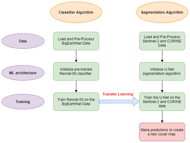
The Resnet-50 CNN classifier architecture won the ImageNet Large Scale Visual Recognition Challenge (ILVRC) in 2015 (Russakovsky et al., 2015) and so is adept at solving image classification problems. The classifier was already pre-trained on the ImageNet (Deng et al., 2009) dataset, which consists of approximately 14 million images divided into roughly 21 000 different classes. This classifier was retrained using the BigEarthNet satellite image data and labels (Sect. 2.3) and the fastai python library (Howard and Gugger, 2020), with the goal of classifying satellite images according to land-cover classes present in the images. In order to create a new cover map a segmentation algorithm was required to make a land-cover prediction for each pixel in a satellite image. The U-Net segmentation CNN was deployed. This type of model involves an encoder part, where the architecture down-samples an input image while also inferring image features, and a decoder part where the features inferred are up-sampled again and a prediction mask is outputted. The retrained classifier was re-purposed as the encoder part of the algorithm. The U-Net was then trained on satellite segments and corresponding CORINE segments, which act as ground truth outputs. The result, after the algorithm has been trained, is a prediction for each pixel of the input image in the form of a prediction mask of the same size as the input image, in this case 120×120 px.
3.2 Model training
The steps involved in training of the Ulmas-Walsh land-cover predictor are summarised as follows:
-
Re-training the Resnet-50 classifier: the Resnet-50 classifier mentioned in Sect. 3.1 was retrained to infer CORINE labels from the satellite images in the BigEarthNet dataset (Sect. 2.3).
-
Train the U-Net segmentation algorithm: the now re-trained Resnet-50 classifier was installed as the encoder of the U-Net segmentation algorithm (Sect. 3.1). This model was then trained on Sentinel-2 data as the input and CORINE data as the ground truth output. The resulting algorithm was used to create a new land-cover map.
3.3 Primary and secondary models
Following the workflow outlined in Sect. 3.1 and 3.2, the Primary Satellite Segmentation Algorithm, the Primary Ulmas-Walsh Predictor, UWP hereafter, was developed using 5 labels during classifier and segmentation training. These 5 labels were the 5 Primary CORINE land-cover labels.
In order to train the Primary UWP, 2 Sentinel-2 tiles over Ireland were chosen and can be seen in Fig. 3a and b. The training data for the Primary UWP consisted of 16 562 120×120 px satellite segments and the corresponding CORINE land-cover segment for each.
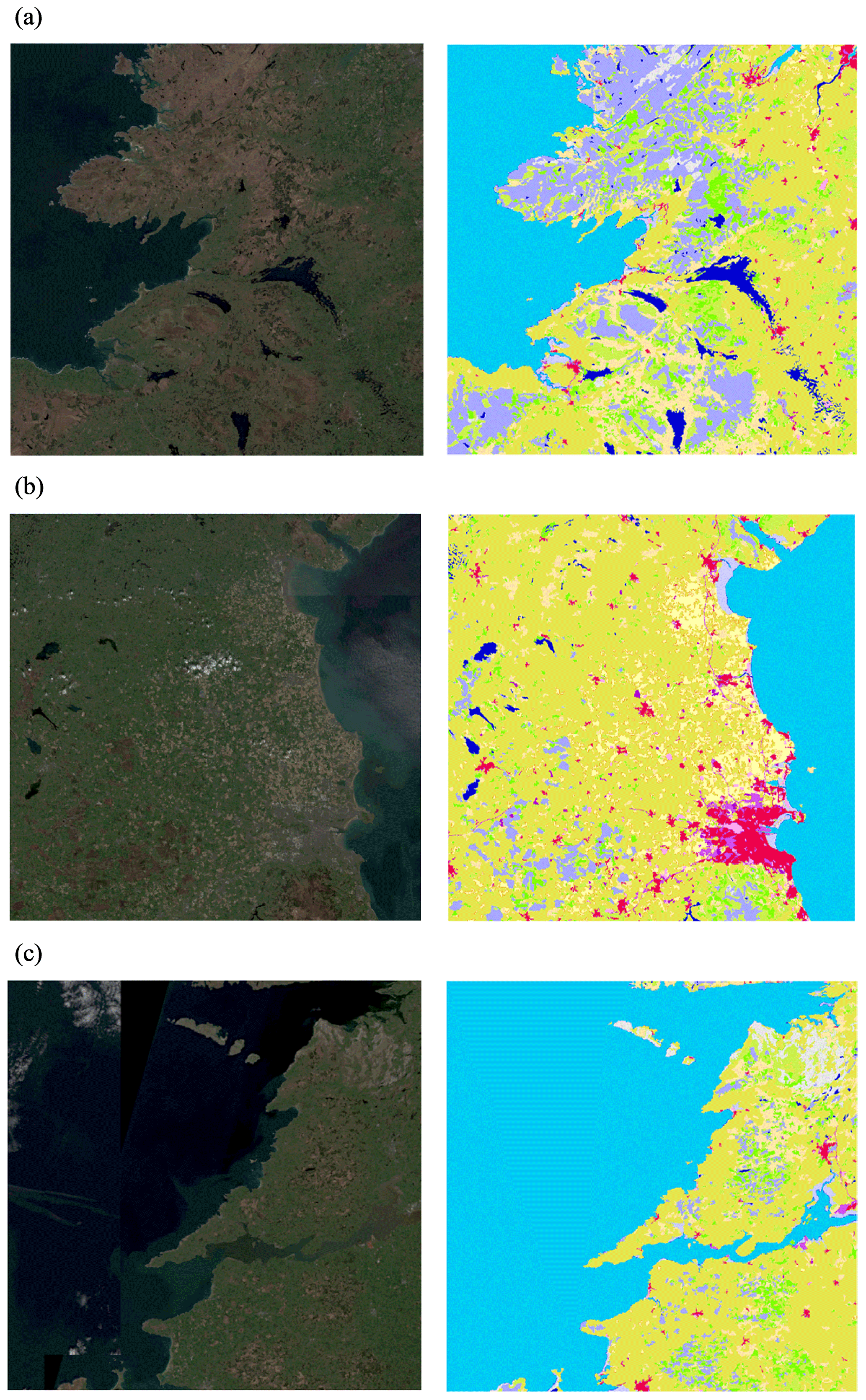
Figure 3Sentinel-2 tiles and corresponding CORINE tiles used to train the Primary and Secondary UWPs. (a) Donegal in the North-West of Ireland (b) Dublin City and its surrounds on the East Coast of Ireland. (c) County Clare on the West Coast of Ireland. The satellite images were produced from ESA remote sensing data.
The Secondary UWP was trained in the same way as the Primary UWP. The only difference was that the Secondary UWP had more training labels, in the form of the 15 secondary CORINE land-cover labels. As there were more labels, more training data was required so as to account for these labels. Some of the secondary labels were not present in the two tiles used to train the Primary UWP, therefore a third tile containing these labels was added to the training data. The Sentinel-2 and CORINE tiles in Fig. 3c were added to the training data as a result. The updated training data consisted of 24 843 120×120 px satellite segments and the corresponding CORINE segments for these satellite areas.
The results are split into two sections. Section 4.1 contains the results of the Primary UWP, while Sect. 4.2 contains the results of the Secondary UWP. In order to compare ECO-SG to CORINE and to both the primary and secondary predicted land-cover maps, the ECO-SG map labels needed to be converted to CORINE labels (see Appendix A for both conversion tables).
The conversion of ECO-SG's labels to the primary CORINE labels was straightforward, the 5 Primary CORINE labels were generic enough to allow for the conversion of each of ECO-SG's land-cover labels to one of these 5 labels without any ambiguity (see Table A1). A statistical comparison and analysis of these maps was possible as a result.
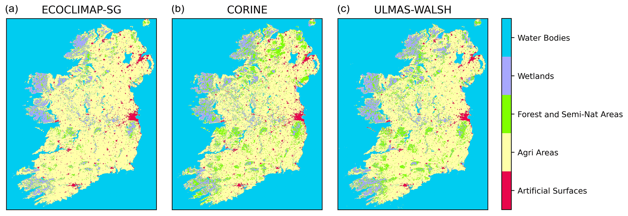
Figure 4Land-cover maps of Ireland: ECO-SG (a), CORINE (b) and the UW map (c). Pixel-wise, ECO-SG was found to be 89.9 % similar to CORINE. The UW map was found to be 92.5 % similar to CORINE.
The conversion of the ECO-SG map labels to CORINE labels in the case of the secondary CORINE labels was not as simple (see Table A2). The ECO-SG labels were successfully converted into 10 of the CORINE secondary labels. However, some of the conversions are open to debate. CORINE prioritises land use and land properties in its labels, whereas ECO-SG is concerned with the effects of land-covers, specifically there perceived surface roughness, on numerical weather prediction, as a result it can be hard to reconcile some of the land-cover labels from ECO-SG with labels in CORINE. This also meant that there were 5 extra labels in both the CORINE map and the Ulmas-Walsh map, hereafter the UW map (trained on CORINE data and labels so therefore has 15 labelling options when the model made pixel-wise predictions), as there are 15 CORINE labels in total. Conclusions from a statistical comparison of the secondary maps could not be drawn as a result as it would not be rigorous or experimentally fair, however other important conclusions, namely the robustness of the method and its favourable characteristics when increasing the number of labels, can be drawn from these results.
4.1 Primary UWP results
To determine how the predicted land-cover map for Ireland, the UW map, performs in comparison to ECO-SG, a reference map had to be used as the control. The ML algorithm was trained using the CORINE land-cover map as it is considered to be 85 % accurate. Since it was the most accurate map available, it was used as the control for comparison purposes in the absence of a freely-available land-cover map based on local datasets covering Ireland.
The versions of ECO-SG, CORINE and the UW map displaying the CORINE primary labels are shown in Fig. 4. Qualitatively, we can see that the the UW map is more alike the CORINE map than ECO-SG as one might expect because the ML algorithm was trained on CORINE data. There appears to be more forest and semi-natural areas present in the UW map than in ECO-SG. Given that one of the issues with ECO-SG in Ireland is that it over-categorises Ireland as pastures, which in this case comes under the agricultural areas label, this is a positive outcome. The qualitative viewpoint is backed up numerically when we compare the overall accuracy of ECO-SG and the UW map with CORINE (Eq. 1).
ECO-SG was found to be 89.9 % similar to CORINE, while the UW map was 92.5 % similar to CORINE.
The proportion of each land-cover in the 3 maps is summarised in Fig. 5. Water Bodies has been omitted from the graph in order to better observe the variations of the land-cover type proportions across the 3 maps. Each map had approximately 50 % water body cover. Appendix B contains 2 tables that give details on the square kilometre coverage and the percentage coverage of each land-cover in the 3 maps. Figure 5 demonstrates that the UW map has proportions more in-line with CORINE, especially in the forest and semi-natural areas category when compared with ECO-SG. Much of the change between ECO-SG and the UW map is that the agricultural-areas proportion shrinks in the UW map and conversely the forest and semi natural areas increase. Artificial surfaces and wetlands have about the same proportion in the 3 maps.
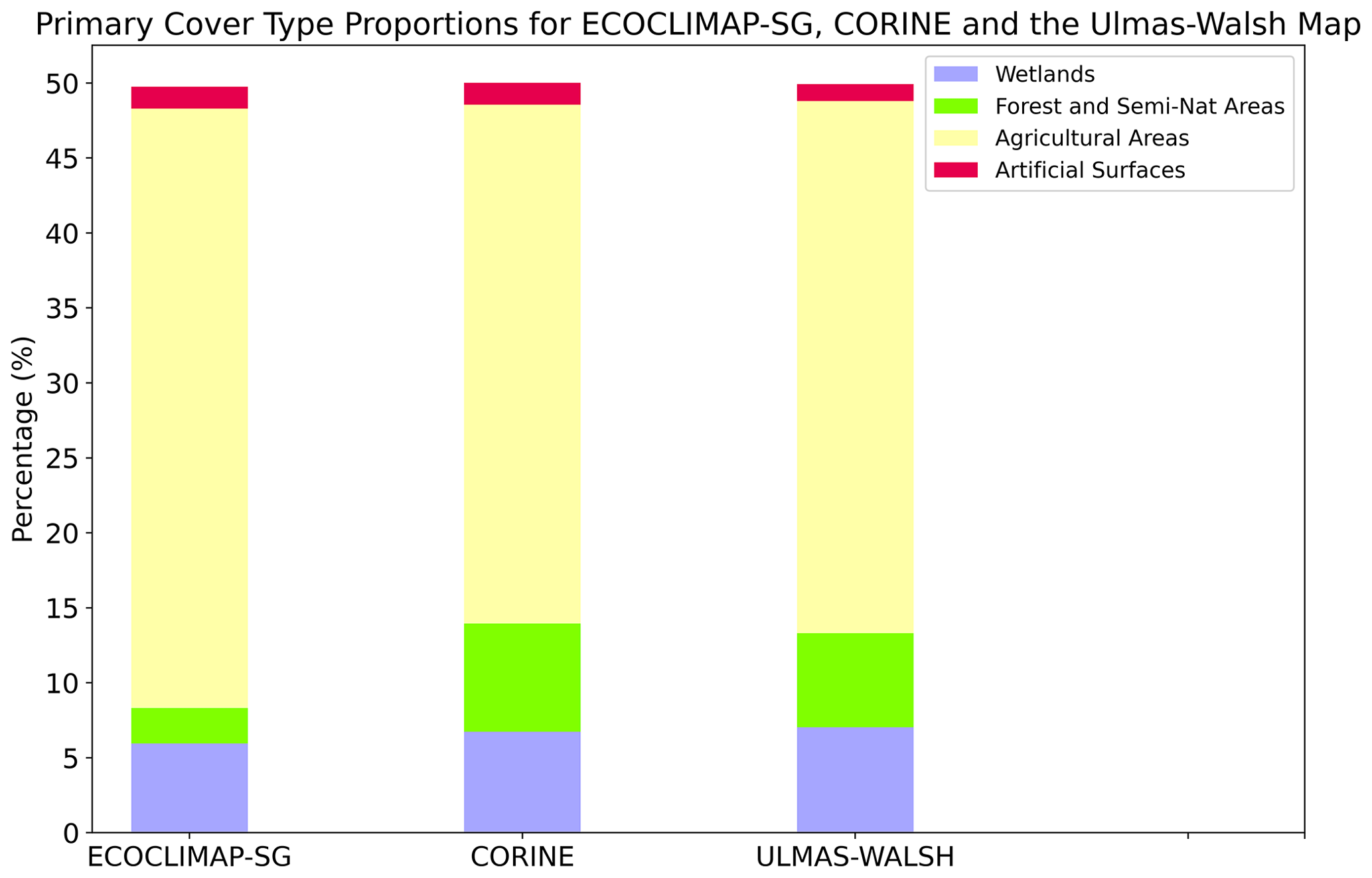
Figure 5Proportion of each of the 4 Primary land-cover types for each of the 3 maps shown in Fig. 4. The Water bodies label is omitted for easier comparison of the terrestrial land-covers.
While having a more accurate proportion of each category in the map is important, the spatial accuracy of each category is most critical. The Jaccard Index metric is a way of gauging this (Eq. 2). The predicted pixels for a land-over label in one map, A1 (ECO-SG or UW) are compared with the true value for that land-cover label in the control, A2 (CORINE). The intersection of the predicted pixels (A1) and the control pixels (A2) for the land-cover label in question are divided by the union of the land-cover label in question in both maps. The resulting value (between 0 and 1) is a metric of how close the prediction is to the control. The closer the value is to 1 the closer the prediction for the land-cover label in question is to the ground truth for that label. The Jaccard index is a common analytical tool in the ML for gauging the quality of ML segmentation algorithms (Ulmas and Liiv, 2020; Ronneberger et al., 2015).
In Fig. 6, an improvement across 3 of the 5 Primary land-cover types can be seen, with the water bodies class giving approximately the same result in each map and the artificial surfaces class is slightly better in ECO-SG than in the UW map when compared with CORINE. The average Jaccard Index per class for ECO-SG when compared with CORINE was found to be 0.61, while the average value was found to be 0.69 when comparing the UW map with CORINE.
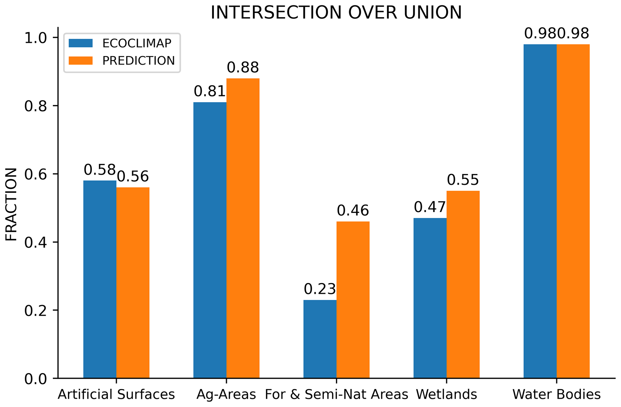
Figure 6Jaccard Index (Intersection Over Union) for the 5 land-cover labels when comparing ECO-SG (blue) and the Ulmas-Walsh map (orange) with CORINE.
So far it has been shown that the UW map is closer in accuracy to CORINE than ECO-SG, in terms of overall pixel-wise accuracy and spatial accuracy. However, it was thought that the UW map potentially correctly categorises some areas that the CORINE map has mislabelled. While the algorithm used to produce the UW map was trained using CORINE data, quite a lot of unseen data (data not used to train the algorithm) were used to produce the full map. Figure 7 shows a number of examples of the UW map compared with ECO-SG and CORINE, along with the satellite image for the areas in question. The top row represents a region of wetland in County Galway in the west of Ireland. The Sentinel-2 image shows a majority wetland area (brown). ECO-SG overestimates the proportion of wetland areas in the image (purple), and CORINE underestimates this area, mislabelling it as forest and semi-natural areas (green). Conversely, the UW map is more comparable to the ground truth Sentinel-2 image. In the second row in Fig. 7 the forestry areas in the Sentinel-2 image (dark green) are only picked up by the UW map (green). The third row represents the Phoenix Park in County Dublin. ECO-SG miscategorises this area as completely urban in extent. CORINE recognises that natural areas are present, but fails to recognise any forestry in the area. However, the UW map has detected the presence of tree coverage in the area. The bottom row represents a small lake in County Clare. This water body is only present in the UW map and is erroneously absent in ECO-SG and CORINE, more than likely a consequence of the data and methods used to create these maps. We see how the UW map is closer to CORINE than ECO-SG, but also that the UW map diverges from the CORINE map in places and correctly picks up on details that are not accounted for in CORINE. Such differences lead to a divergence between the UW map and the CORINE equivalent, which are not quantitatively represented in the statistical analysis above, whereas in reality these differences represent an improvement.
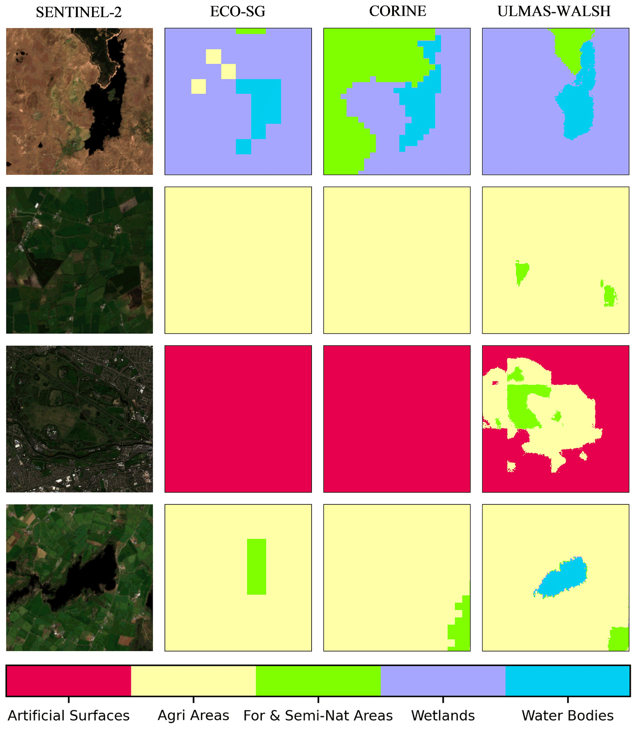
Figure 7Satellite image segments and the corresponding ECO-SG, CORINE and UW cover maps for these images. Row 1 represents a bog in County Galway in the West of Ireland (53.30, −9.34). Row 2 represents an area in County Tipperary in the midlands (52.72, −7.75). Row 3 represents the Phoenix park and its surrounds in County Dublin in the East (53.35, −6.33) Row 4 represents a lake in County Galway in the west (53.10, −8.87). The fully labelled ECO-SG and ESA-CCI land-cover maps for these satellite images can be found in Appendix C. The satellite images were produced from ESA remote sensing data.
Figure 7 also qualitatively demonstrates another key feature of the ML algorithm, improved pixel-wise resolution. ECO-SG has a resolution of 300×300 m per pixel and CORINE is 100×100 m per pixel, the UW map demonstrates a resolution of 10×10 m per pixel. This is a natural consequence of the resolution of the Sentinel-2 satellite images, which have a 10×10 m resolution. Since predictions are made pixel wise, the output map has a resolution of 10×10 m.
One of the potential advantages of using a ML model to create a land-cover map is that it can be updated on a semi-regular basis, with the caveat that there are cloud free images available. Some land-cover phenomena only manifest themselves during certain times of the year, such as Turloughs, which are seasonal lakes, commonly found in the West of Ireland. Figure 8 shows one such Turlough known as Lough Funshinagh, located in County Roscommon in the mid-West of Ireland. Figure 8 shows two satellite images, one from (a) April 2020 when the Lake is present and one from (b) August 2020 when it is close to empty and the corresponding prediction yielded by the primary UWP for each satellite image. The primary UWP yields different cover maps which reflect the land-cover change that has occurred, in this case that the lake is present in April and has almost totally diminished in August.
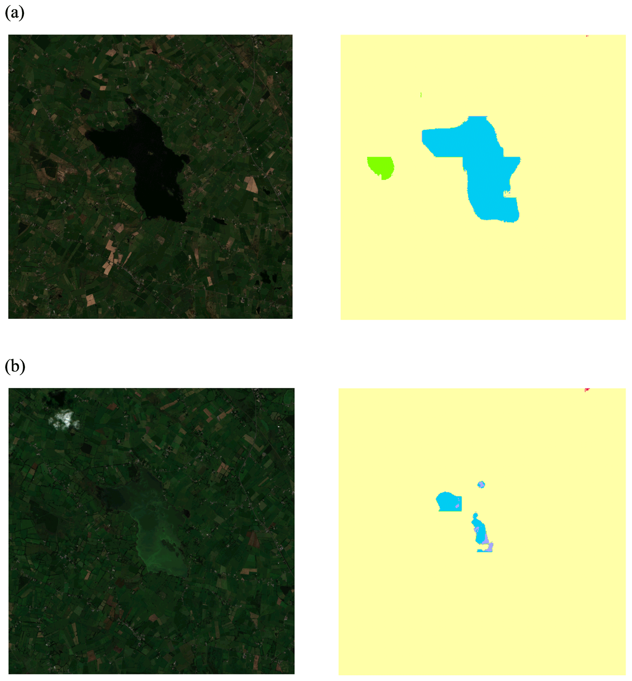
Figure 8Lough Funshinagh, a Turlough (seasonal lake) in the West of Ireland (53.51, −8.1) in (a) April 2020 and (b) August 2020, obtained from Sentinel-2 satellite images, with the corresponding UW map for both. The satellite images were produced from ESA remote sensing data.
4.2 Secondary UWP results
A secondary UWP was trained using the 15 CORINE secondary labels, to see if an algorithm could be trained that maintains the performance of the primary UWP but with more labels, which would be necessary for any future meteorological land-cover map. Due to the issues outlined at the start of Sect. 4, not all of the metrics that were used in Sect. 4.1 to gauge the accuracy and precision of the primary UW map, were used to analyse the secondary UW map. The overall pixel-wise accuracy was once again compared, along with the Jaccard Index for land-cover labels present in all 3 maps. Qualitative comparisons were also made demonstrating the improved accuracy, resolution and pliability of the secondary UW map when compared with ECO-SG and CORINE.

Figure 9Land-cover maps of Ireland for ECO-SG, CORINE and the UW map. Pixel-wise, ECO-SG was found to be 82.4 % similar to CORINE. The UW map was found to be 86.4 % similar to CORINE.
Figure 9 shows the ECO-SG, CORINE and UW maps with 15 potential cover types listed. The UW map qualitatively still performs well despite the extra amount of labels. The UW map does have an issue where some areas of marine waters (light blue) off of the the west coast of Ireland are labelled as continental waters (dark blue), and some areas of continental waters are being labelled as marine waters. This is due to the similarity of fresh water and sea water in RGB satellite images. Quantitatively, ECO-SG was 82.4 % like CORINE and the UW map was 86.4 % like CORINE, which demonstrates that despite the addition of 10 extra labels, the UW map still performs to a high level. There is a caveat with the ECO-SG result, only 10 of the CORINE labels were determined to be present in ECO-SG, meaning that 5 were not present at all, which affects the accuracy score. The 5 missing labels in ECO-SG account for 4.26 % of the CORINE map and so it could be argued that the accuracy gap between ECO-SG and the CORINE map is accounted for by this disparity in the labelling. However, it could also make the accuracy worse; on this point there is not any clarity.
To get an idea of the spatial accuracy of each of the land-cover categories, the Jaccard Index was once again deployed. Figure 10 shows the Jaccard index for 8 of the 15 CORINE labels. The 5 missing from ECO-SG were discounted here, along with shrub where the proportion in ECO-SG was close to 0 % and permanent crops where the value was 0 %. The 8 labels remaining account for ∼92 % of the CORINE map. Across the 8 labels, the UW map has higher values for the Jaccard index in 6 of them, the exceptions being continental waters and marine waters, which further highlights the issues visible in Fig. 9. The average Jaccard index for ECO-SG was found to be 0.5 and the average for the UW map was found to be 0.55. The relatively small difference between the average Jaccard index is mainly due to the issue highlighted earlier between continental waters and marine waters. When continental waters is removed, the ECO-SG Jaccard index falls to 0.47 while UW equivalent rises to 0.58 on average, which is closer to the 0.69 obtained with the primary labels.
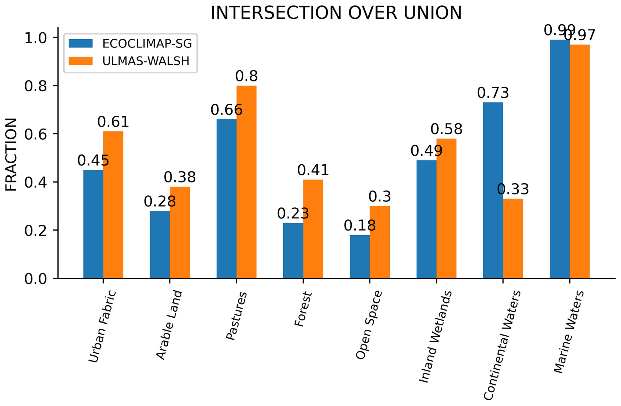
Figure 10Jaccard Index (Intersection Over Union) for 8 of the 15 land-cover classes when comparing ECO-SG (blue) and the Ulmas-Walsh map (orange) with CORINE.
As with the Primary UWP (Fig. 7), it was demonstrated that the secondary UWP also deviates from CORINE, and picks up on areas that CORINE labels incorrectly (see Fig. 11). The same areas as in Fig. 7 when analysing the primary UW map were used to analyse the secondary UW map. Much of the same improvements can be seen in the four areas for the secondary UW map as were seen in the primary UW map, which demonstrates that the predictions deviate from CORINE and pick up on land-cover types that were not labelled in CORINE, even with more labels in the secondary UWP. The third row depiction of the Phoenix park in county Dublin yields an interesting prediction when compared with CORINE. CORINE labels the Phoenix park as being an Urban Green Area, which it is, however the prediction made by the UW predictor has a mixture of labels in this area, such as Pastures and Forest as well as Urban Green Areas. By definition, an urban green area is a natural area in an urban setting and so would contain characteristics of a number of natural land-covers, such as Pastures and Forests. Graphically then these labels would look much the same and hence the mislabelling when compared to the CORINE ground truth, although it is not a completely inaccurate mislabelling as the covers imply the same thing in reality. These examples also once again demonstrate the improved resolution of the UW map when compared with ECO-SG and CORINE, thanks to the resolution of the Sentinel-2 data used to obtain the predicted maps.
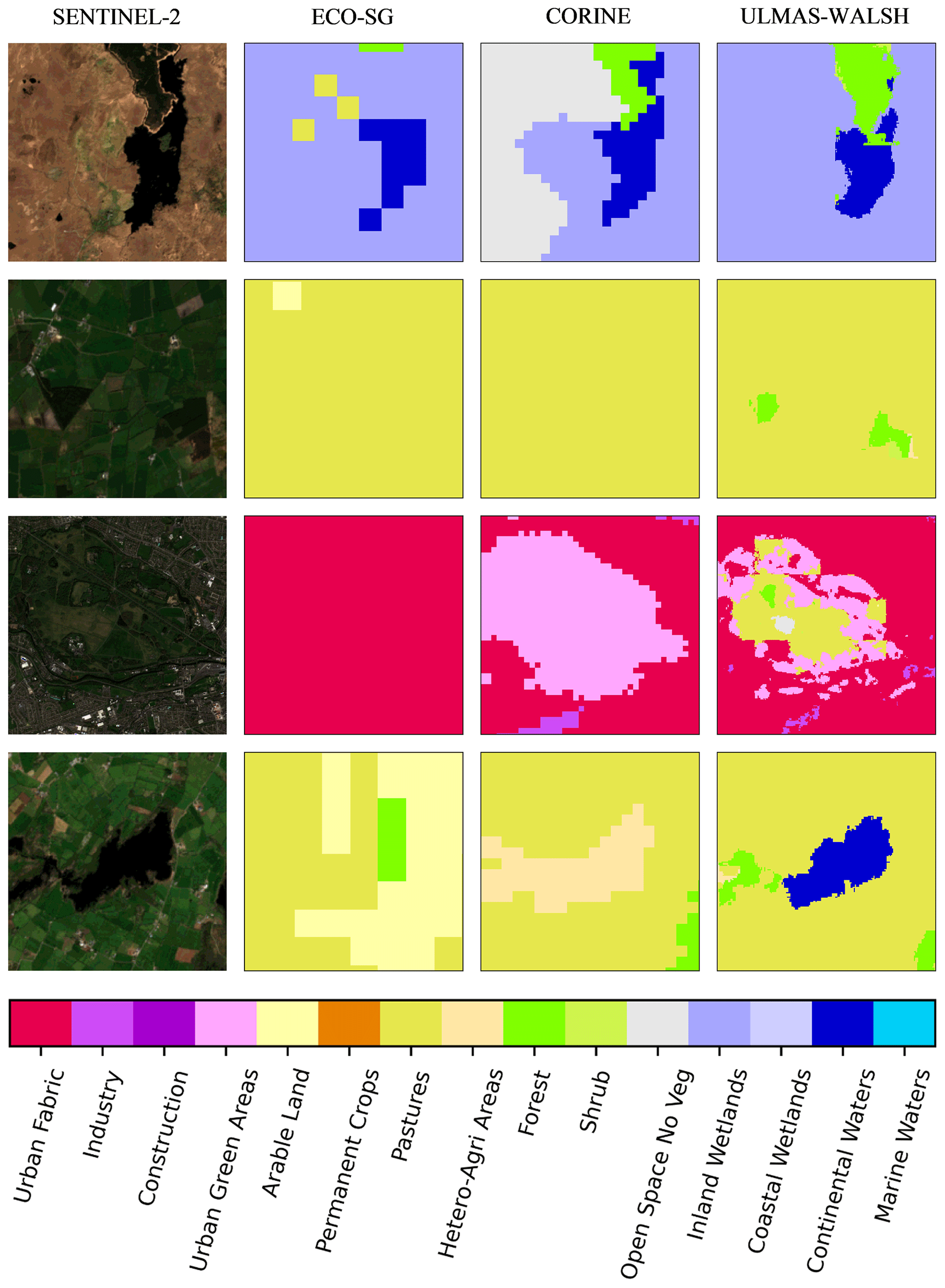
Figure 11Satellite image segments and the corresponding ECO-SG, CORINE and UW cover maps for these images with secondary CORINE land-cover labels. The same areas as in Fig. 7 are shown. The satellite images were produced from ESA remote sensing data.
The application of the UW predictor to the secondary CORINE labels does not result in the performance of the algorithm reducing relative to the primary UW predictor, despite the increased complexity of the task given the addition of more labels. The satellite images of the Turlough, Lough Funshinagh, as previously seen in Fig. 8, at different times of the year once again yield accurate predictions for the two very different environments present, the result of which can be found in Appendix D.
The Ulmas-Walsh (UW) map, obtained via a ML algorithm, has been shown to be more accurate (Primary UWP) or at least as accurate (Secondary UWP) as ECO-SG when compared with the CORINE land-cover map. As well as that, the algorithms demonstrate an ability to pick up on areas mislabelled in the CORINE map for Ireland.
The direct pixel accuracy of both of the maps created when compared to CORINE came out at 92.5 % and 86.4 % which is superior to the appropriately labelled ECO-SG maps for each model (89.9 % and 82.4 %). The two UW maps had on average a higher Jaccard Index, which measures spatial accuracy as well as proportional accuracy, a key indication that the UW map is more accurate than ECO-SG. It has also been shown that despite being trained on CORINE data, the algorithm produces land-cover label predictions which differ from those of CORINE, and when both maps are compared with satellite images, we see areas which CORINE mislabelled and the UW map correctly labelled (see Figs. 7 and 11).
The primary and secondary UW maps also show an improved pixel-wise resolution compared to both ECO-SG (300×300 m per pixel) and CORINE (100×100 m per pixel) of 10×10 m, a consequence of the Sentinel-2 images having a resolution of 10×10 m, and the algorithm's labelling process occurring on a per pixel basis. Given that the Numerical weather prediction model, HARMONIE-AROME, will require higher input resolution in future cycles, this ML based algorithmic method offers a potential path to a process which will produce higher resolution land-cover maps.
There are a number of advantages to applying a ML algorithm, akin to what has been developed in this work. Once the ML algorithm had been developed, obtaining predictions from the algorithm and assembling the map was a relatively quick process. From start to finish, this process of obtaining predictions for the satellite images and then reassembling these predictions to produce a land-cover map for Ireland takes about 1 d, once the full workflow had been developed, the rate limiting step being computing power. The use of supercomputers, such as those at ECMWF would speed this process up considerably. Acquiring data is another rate limiting step, in order to create a new map a full set of cloud free satellite images is required and this might take a number of days to accumulate. This is in stark contrast to other land-cover maps, such as CORINE, which has an updated release every 6 years. The ML algorithm produced here allows for a map that can be updated frequently, allowing for seasonal surface changes, as demonstrated by the seasonal lake results in Figs. 8 and D1. This could be expanded to include seasonal changes in crops which effect surface roughness. ECO-SG and CORINE do not demonstrate such flexibility. The development of maps such as CORINE are of critical importance for the development of supervised ML algorithms, such as what has been discussed in this paper. Without a large volume of easily accessible high quality data, Sentinel-2 images and the CORINE land-cover map in this case, such algorithms would not be possible.
A ML algorithm offers a universal way of improving a land-cover map. Attempts to improve the quality of land-cover maps revolve around the use of national data, which differs from jurisdiction to jurisdiction and so any improvements are not homogeneous. The homogeneity of map quality is an important characteristic to have in a meteorological land-cover map, differences in quality between jurisdictions results in artificial borders which has a knock-on adverse effect on numerical weather predictions, caused by these artificial jumps in surface fluxes. A ML algorithm relies on the data provided to it during its training process to make its predictions. A cross-jurisdictional map could then be produced by providing cross-jurisdictional data, which is easily accessible via Sentinel-2 satellite images and, in the case of Europe, the CORINE land-cover map. The scope of data that could be used is not limited to these resources either, if there are superior local datasets available, they could be harnessed to train an algorithm also.
A ML algorithm also provides full open access control for the meteorological community to use it and develop it as appropriate into the future, be that adding extra labels to the map or adding new jurisdictions etc. These algorithms are easily initiated using open access programming languages such as python, and most importantly, the data used to produce this algorithm is also obtainable from open access sources.
In the immediate future, work will revolve around further analysis of the maps produced in this work, through the evaluation of other parameters related to meteorological land-cover maps, such as building heights, urban densities and tree heights.
Looking to further future work that could be potentially undertaken, the scope is wide. The ML algorithm developed here is large and complex in terms of its size, and was developed using well known architectures and well established practises in the field of ML, such as the U-Net architecture and the transfer learning technique. The data selection process however, was not sophisticated. Regions with the relevant covers present in them were chosen, with no statistical survey done outside of a qualitative assessment. A rigorous data selection process, which accounts for all land-covers in a balanced way, may yield improvements. Future work should also involve expanding the number of labels in the map further, potentially the tertiary CORINE land-cover map, which contains 44 labels. Rigorous data selection and balanced label proportions becomes more important as more labels are added to any ML algorithm, and so any undertaking with a significant amount of labels should make quality data selection a priority. Any future work should also investigate the application of such an algorithm in multiple jurisdictions, possibly in UWC-West nations, which Ireland is a member of, before extending to the other UWC nations, and long term to the ACCORD nations, something that will be necessary if a ML produced map is to be used widely in producing land-cover maps in the shared ALADIN-HIRLAM numerical weather prediction system (see Appendix E for more information on UWC-West, UWC and ACCORD). Future work could also investigate the possibility of seasonal updates for relevant seasonal covers, such as crops, seasonal lakes, flood plains etc, which would provide a more accurate near real-time surface roughness estimate in regions with such seasonal land-covers. The issue of mislabelling between the marine waters and continental waters covers in the secondary UW map gives scope for future work involving other non-visible Sentinel-2 bands that could potentially distinguish between freshwater and salt water bodies better. This applies in general too, having more Sentinel-2 bands involved in general should equate to better results, as extra bands give the algorithm more data to discern differences between land-covers.
Table A1Conversion table for ECO-SG labels to primary CORINE labels.
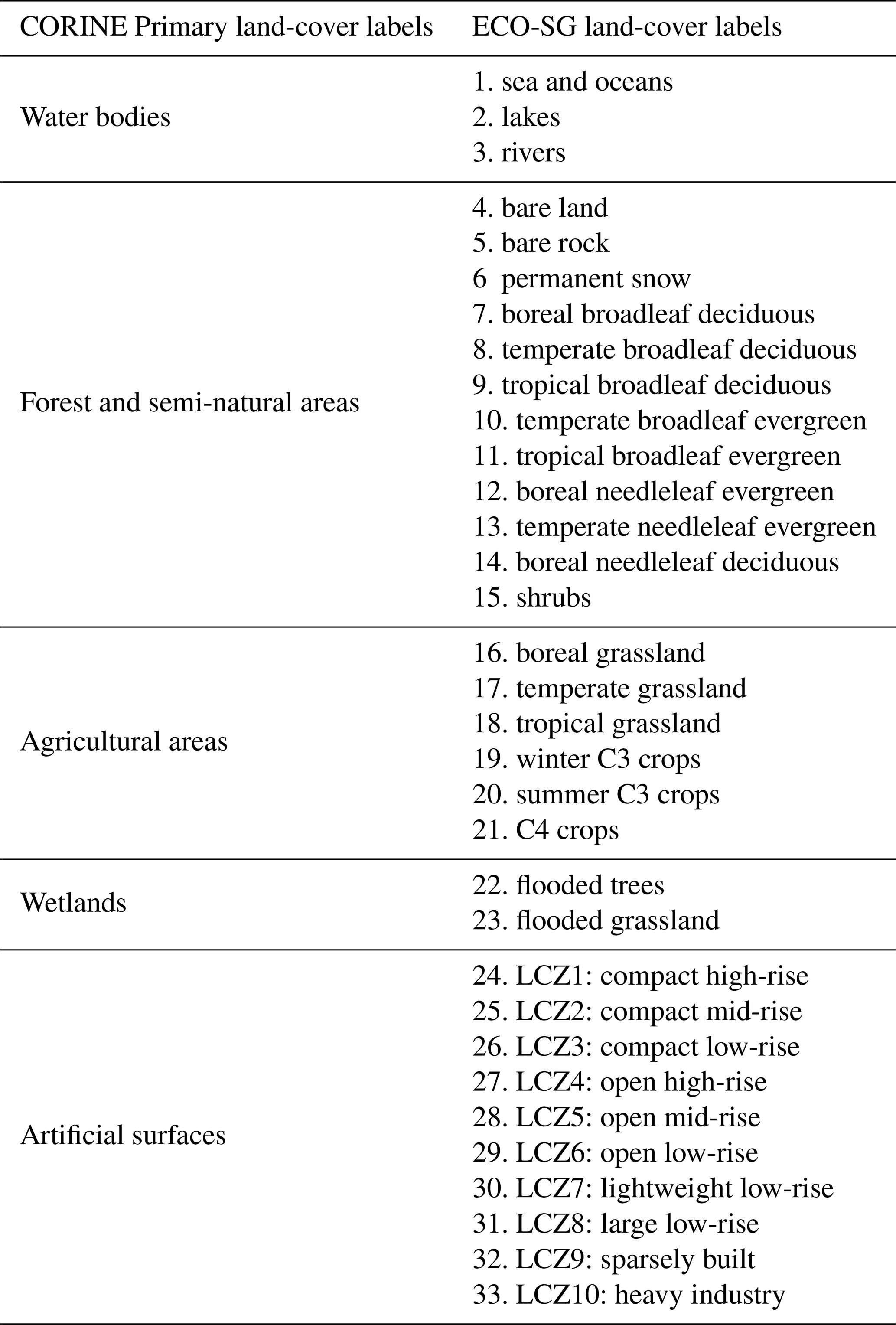
Table A2Conversion table for ECO-SG labels to secondary CORINE labels.
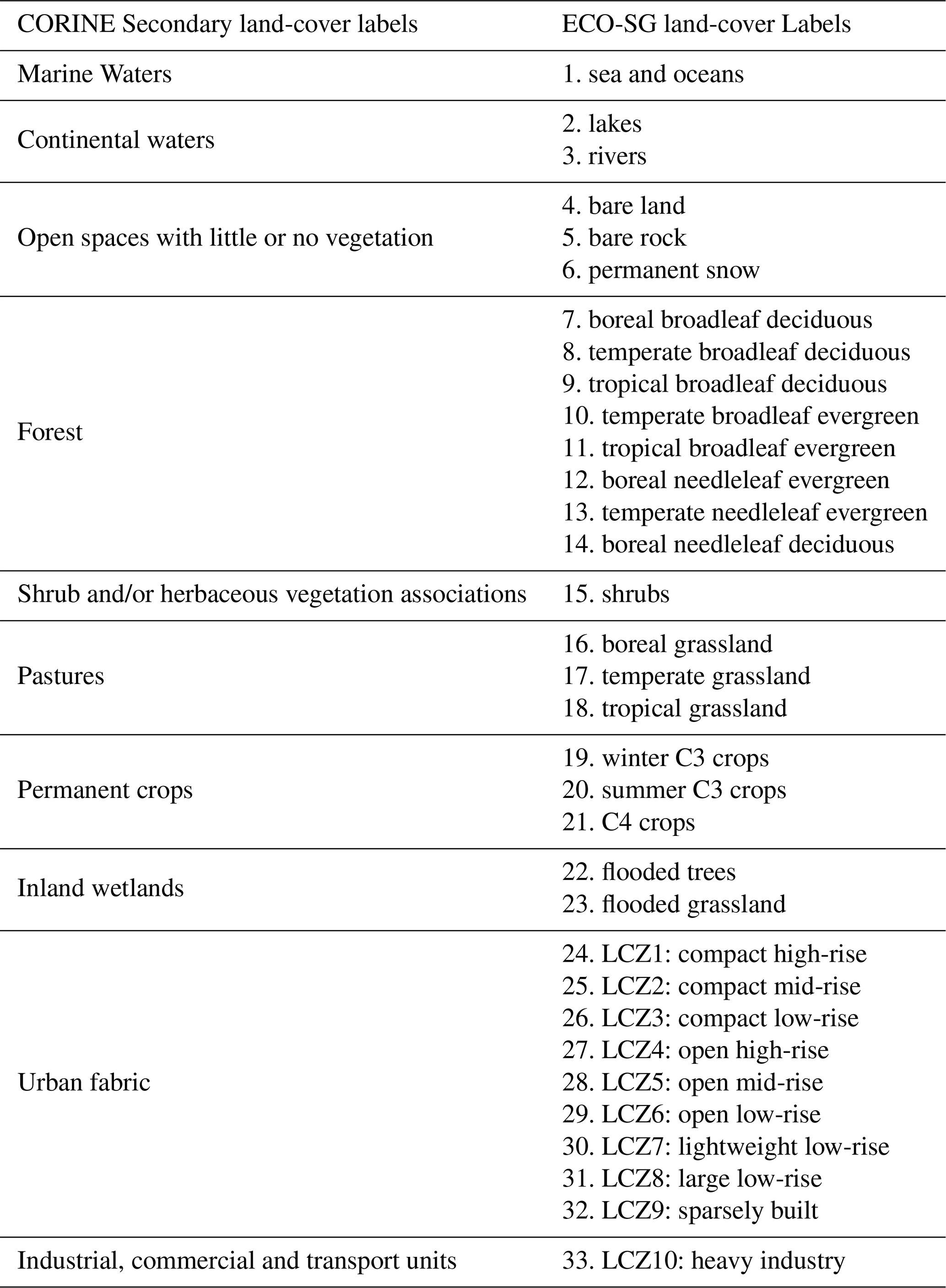
Table B1Proportion of each of the 5 categories present in ECO-SG, CORINE and the UW map in square kilometres.

Table B2Proportion of each of the 5 categories present in ECO-SG, CORINE and the UW map in percentage terms.
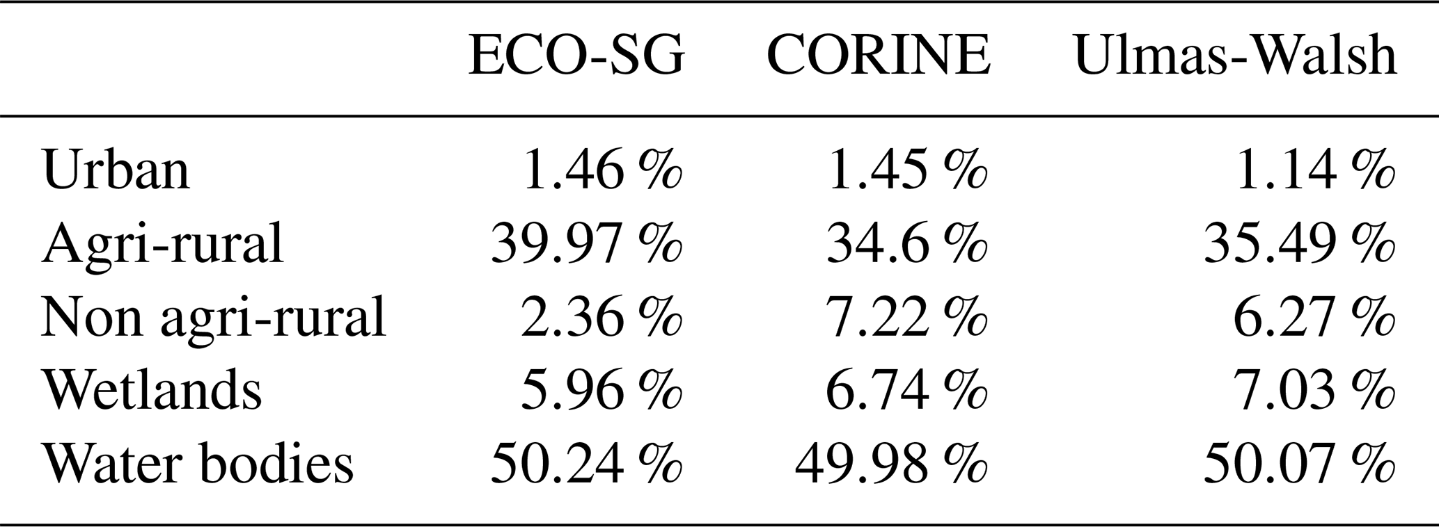
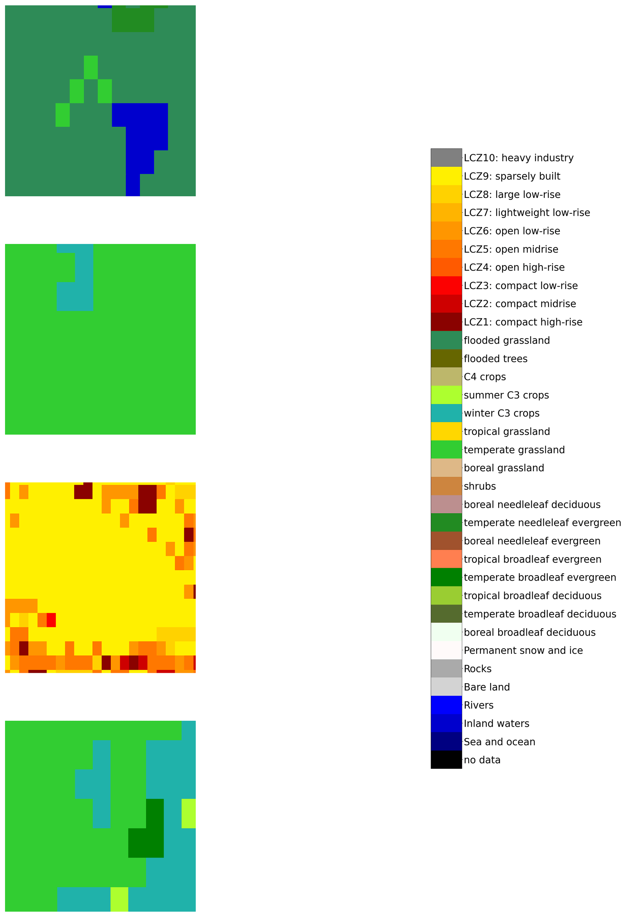
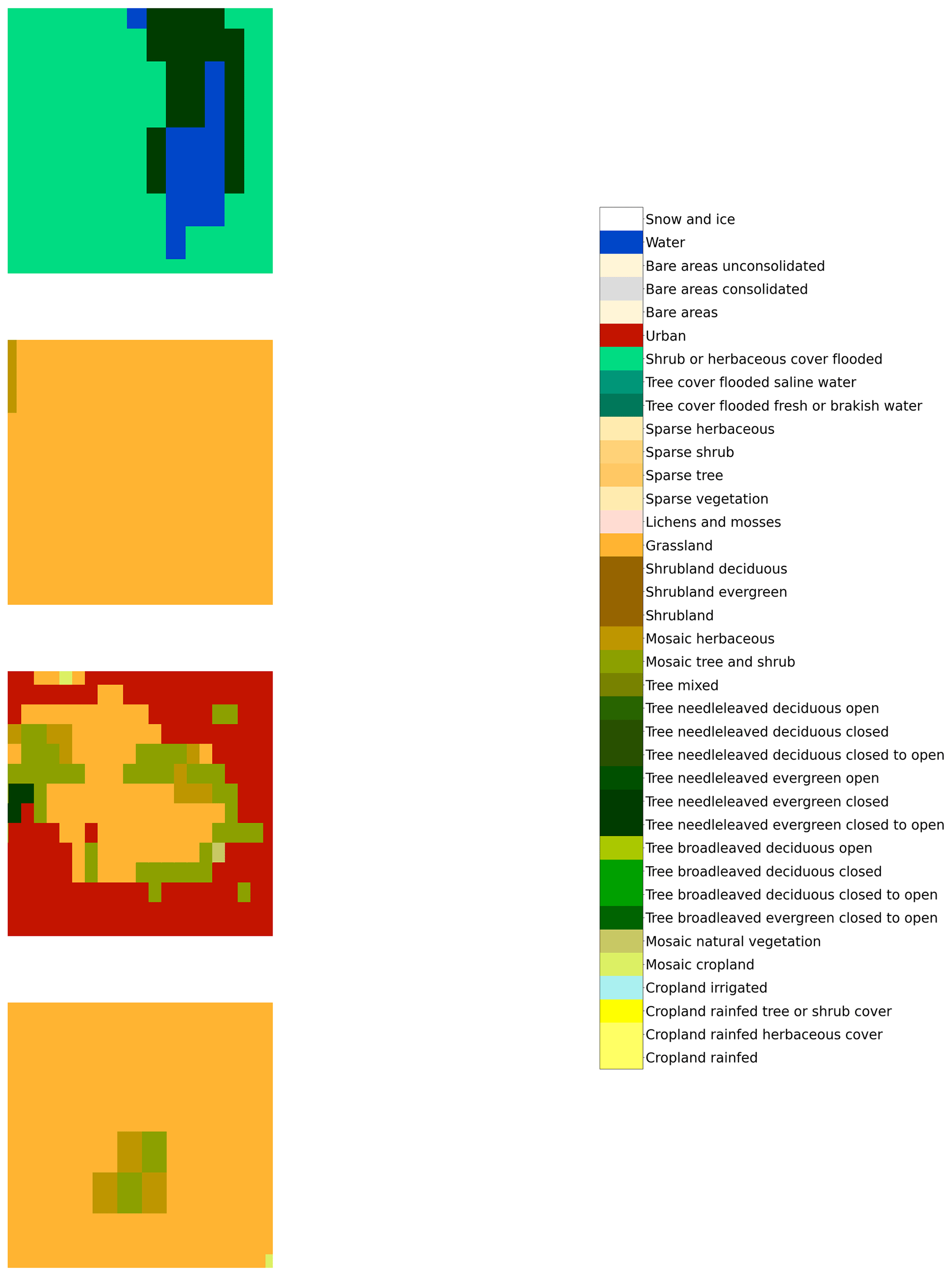

Figure D1Lough Funshinagh, a Turlough (seasonal lake) in the West of Ireland in (a) April 2020 and (b) August 2020, obtained from Sentinel-2 satellite images, with the corresponding secondary UW map for both. The satellite images were produced from ESA remote sensing data.
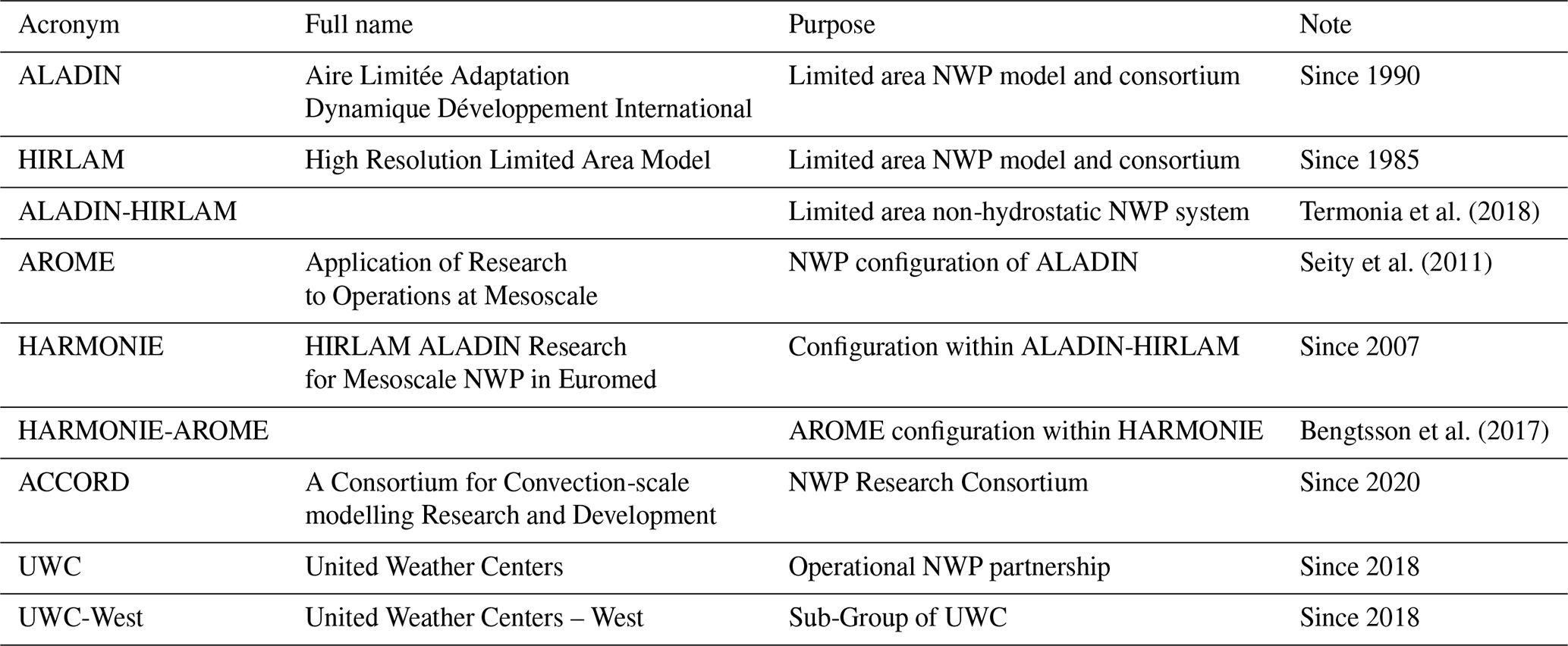
Table E1Further Details on various NWP models, configurations and consortia mentioned in this work.
Code and results data available upon request. The data used to obtain the results is open-source and available at the following web addresses: CORINE land-cover dataset: https://land.copernicus.eu/pan-european/corine-land-cover (last access: 30 April 2021) (Copernicus, 2021a), Sentinel-2 Satellite Data: https://scihub.copernicus.eu/ (last access: 30 April 2021) (Copernicus, 2021b), BigEarthNet: http://bigearth.net/ (last access: 30 April 2021) (BigEarthNet, 2021).
All authors contributed to the writing of this paper. The original CNN algorithm was written by PU and modified by EW for use over Ireland. The simulations were run by EW with input from GB on manipulation of datasets, projections etc.
The authors declare that they have no conflict of interest.
This article is part of the special issue “Applied Meteorology and Climatology Proceedings 2020: contributions in the pandemic year”.
This publication has emanated from research conducted with the financial support of Science Foundation Ireland under grant no. 18/CRT/6049.
This paper was edited by Balázs Szintai and reviewed by two anonymous referees.
Ballabio, C., Panagos, P., and Monatanarella, L.: Mapping topsoil physical properties at European scale using the LUCAS database, Geoderma, 261, 110–123, https://doi.org/10.1016/j.geoderma.2015.07.006, 2016. a
Bari, D. and Ouagabi, A.: Machine-learning regression applied to diagnose horizontal visibility from mesoscale NWP model forecasts, SN Appl. Sci., 2, 1–13, https://doi.org/10.1007/s42452-020-2327-x, 2020. a
Bartholomé, E. and Belward, A. S.: GLC2000: a new approach to global land cover mapping from Earth observation data, Int. J. Remote Sens., 26, 1959–1977, https://doi.org/10.1080/01431160412331291297, 2005. a
Båserud, L., Lussana, C., Nipen, T. N., Seierstad, I. A., Oram, L., and Aspelien, T.: TITAN automatic spatial quality control of meteorological in-situ observations, Adv. Sci. Res., 17, 153–163, https://doi.org/10.5194/asr-17-153-2020, 2020. a
Bengtsson, L., Andrae, U., Aspelien, T., Batrak, Y., Calvo, J., de Rooy, W., Gleeson, E., Hansen-Sass, B., Homleid, M., Hortal, M., Ivarsson, K.-I., Lenderink, G., Niemelä, S., Nielsen, K. P., Onvlee, J., Rontu, L., Samuelsson, P., Muñoz, D. S., Subias, A., Tijm, S., Toll, V., Yang, X., and Køltzow, M. Ø.: The HARMONIE–AROME Model Configuration in the ALADIN–HIRLAM NWP System, Mon. Weather Rev., 145, 1919–1935, https://doi.org/10.1175/mwr-d-16-0417.1, 2017. a, b, c
Bertini, F., Brand, O., Carlier, S., Del Bello, U., Drusch, M., Duca, R., Fernandez, V., Ferrario, C., Ferreira, M., Isola, C., Kirschner, V., Laberinti, P., Lambert, M., Mandorlo, G., Marcos, P., Martimort, P., Moon, S., Oldeman, P., Palomba, M., and Pineiro, J.: Sentinel-2 ESA's Optical High-Resolution Mission for GMES Operational Services, Remote Sens. Environ., 120, 25–36, 2012. a, b
Bessardon, G. and Gleeson, E.: Using the best available physiography to improve weather forecasts for Ireland, in: Challenges in High Resolution Short Range NWP at European level including forecaster-developer cooperation, European Meteorological Society, Lyngby, available at: https://presentations.copernicus.org/EMS2019/EMS2019-702_presentation.pdf (last access: 30 Apirl 2021), 2019. a
BigEarthNet: About BigEarthNet, available at: http://bigearth.net/, last access: 30 April 2021. a
Cawkwell, F., Raab, C., Barrett, B., Green, S., and Finn, J.: TaLAM: Mapping Land Cover in Lowlands and Uplands with Satellite Imagery, Tech. rep., Environmental Protection Agency, available at: http://www.epa.ie/pubs/reports/research/land/Research_Report_254.pdf (last access: 30 Apirl 2021), 2018. a, b
Chevallier, F., Morcrette, J. J., Chéruy, F., and Scott, N. A.: Use of a neural-network-based long-wave radiative-transfer scheme in the ECMWF atmospheric model, Q. J. Roy. Meteorol. Soc., 126, 761–776, https://doi.org/10.1002/qj.49712656318, 2000. a
CNRM: Wiki – ECOCLIMAP-SG – CNRM Open Source Site, available at: https://opensource.umr-cnrm.fr/projects/ecoclimap-sg/wiki (last access: 30 Apirl 2021), 2018. a, b
Connolly, J.: Mapping land use on Irish peatlands using medium resolution satellite imagery, Irish Geogr., 51, 187–204, 2018. a
Copernicus: CORINE Land Cover, available at: https://land.copernicus.eu/pan-european/corine-land-cover (last access: 30 April 2021), 2021a. a
Copernicus: Copernicus Open Access Hub, available at: https://scihub.copernicus.eu/ (last access: 30 April 2021), 2021b. a
Deng, J., Dong, W., Socher, R., Li, L.-J., Li, K., and Fei-Fei, L.: ImageNet: A Large-Scale Hierarchical Image Database, in: CVPR09, 20–25 June 2009, Miami, Florida, 2009. a
de Vos, L. W., Leijnse, H., Overeem, A., and Uijlenhoet, R.: Quality Control for Crowdsourced Personal Weather Stations to Enable Operational Rainfall Monitoring, Geophys. Res. Lett., 46, 8820–8829, https://doi.org/10.1029/2019GL083731, 2019. a
Doms, G., Förstner, J., Heise, E., Herzog, H.-J., Mironov, D., Raschendorfer, M., Reinhardt, T., Ritter, B., Schrodin, R., Schulz, J.-P., and Vogel, G.: Part II: Physical Parameterization, in: A Description of the Nonhydrostatic Regional COSMO Model, November, COSMO (Consortium for Small-Scale Modelling), Deutscher Wetterdienst, p. 152, 2013. a
Dueben, P. D. and Bauer, P.: Challenges and design choices for global weather and climate models based on machine learning, Geosci. Model Dev., 11, 3999–4009, https://doi.org/10.5194/gmd-11-3999-2018, 2018. a
ECMWF: Part IV: Physical Processes, in: IFS Documentation CY47R1, June, 1–82, available at: https://www.ecmwf.int/node/19748 (last access: 30 April 2021), 2020. a
European Environment Agency: Copernicus Land Service – Pan-European Component: CORINE Land Cover, available at: https://www.eea.europa.eu/data-and-maps (last access: 30 April 2021), 2017. a, b, c, d
European Space Agency: Land Cover CCI Product User Guide Version 2.0, available at: http://maps.elie.ucl.ac.be/CCI/viewer/download/ESACCI-LC-Ph2-PUGv2_2.0.pdf (last access: 30 April 2021), 2017. a, b
Faroux, S., Kaptué Tchuenté, A. T., Roujean, J.-L., Masson, V., Martin, E., and Le Moigne, P.: ECOCLIMAP-II/Europe: a twofold database of ecosystems and surface parameters at 1 km resolution based on satellite information for use in land surface, meteorological and climate models, Geosci. Model Dev., 6, 563–582, https://doi.org/10.5194/gmd-6-563-2013, 2013. a, b, c
Green, S.: ILMO: Irish Land Mapping Observatory, available at: https://www.teagasc.ie/media/website/publications/2016/6405-ILMO.pdf (last access: 30 April 2021), 2015. a
Grönquist, P., Yao, C., Ben-Nun, T., Dryden, N., Dueben, P., Li, S., and Hoefler, T.: Deep Learning for Post-Processing Ensemble Weather Forecasts, available at: http://arxiv.org/abs/2005.08748 (last access: 30 April 2021), 2020. a
He, K., Zhang, X., Ren, S., and Sun, J.: Deep Residual Learning for Image Recognition, in: Proceedings of the IEEE Conference on Computer Vision and Pattern Recognition (CVPR), 27–30 June 2016, Las Vegas, Nevada, 770–778, 2015. a
Hengl, T., Mendes de Jesus, J., Heuvelink, G. B. M., Ruiperez Gonzalez, M., Kilibarda, M., Blagotić, A., Shangguan, W., Wright, M. N., Geng, X., Bauer-Marschallinger, B., Guevara, M. A., Vargas, R., MacMillan, R. A., Batjes, N. H., Leenaars, J. G. B., Ribeiro, E., Wheeler, I., Mantel, S., and Kempen, B.: SoilGrids250m: Global gridded soil information based on machine learning, PLOS ONE, 12, e0169748, https://doi.org/10.1371/journal.pone.0169748, 2017. a, b
Howard, J. and Gugger, S.: Fastai: A Layered API for Deep Learning, Information, 11, 108, https://doi.org/10.3390/info11020108, 2020. a
Hu, X., Shi, L., Lin, L., and Magliulo, V.: Improving surface roughness lengths estimation using machine learning algorithms, Agr. Forest Meteorol., 287, 107956, https://doi.org/10.1016/j.agrformet.2020.107956, 2020. a
Jaffrain, G.: Corine Landcover 2012 Final Validation Report, Copernicus land monitoring, p. 214, available at: https://land.copernicus.eu/user-corner/technical-library/clc-2012-validation-report-1 (last access: 30 April 2021), 2017. a, b
Jones, N.: How machine learning could help to improve climate forecasts, Nature, 548, 379–380, 2017. a
Jung, T., Ruprecht, E., and Wagner, F.: Determination of Cloud Liquid Water Path over the Oceans from Special Sensor Microwave/Imager (SSM/I) Data Using Neural Networks, J. Appl. Meteorol., 37, 832–844, https://doi.org/10.1175/1520-0450(1998)037<0832:DOCLWP>2.0.CO;2, 1998. a
Karstens, C. D., Stumpf, G., Ling, C., Hua, L., Kingfield, D., Smith, T. M., Correia, J., Calhoun, K., Ortega, K., Melick, C., and Rothfusz, L. P.: Evaluation of a probabilistic forecasting methodology for severe convective weather in the 2014 hazardous weather testbed, Weather Forecast., 30, 1551–1570, https://doi.org/10.1175/WAF-D-14-00163.1, 2015. a
Karstens, C. D., Stumpf, G. J., Ling, C., Kingfield, D. M., Correia Jr., J., LaDue, D., Kuhlman, K. M., Meyer, T. C., Smith, T. M., Cintineo, J. L., Melick, C. J., and Rothfusz, L. P.: Forecaster Decision-Making with Automated Probabilistic Guidance in the 2015 Hazardous Weather Testbed Probabilistic Hazard Information Experiment, in: Fourth Symposium on Building a Weather-Ready Nation: Enhancing Our Nation's Readiness, Responsiveness, and Resilience to High Impact Weather Event, American Meteorological Society, New Orleans, available at: https://ams.confex.com/ams/96Annual/webprogram/Paper286854.html (last access: 30 April 2021), 2016. a
Krasnopolsky, V. M. and Lin, Y.: A neural network nonlinear multimodel ensemble to improve precipitation forecasts over continental US, Adv. Meteorol., 2012, 649450, https://doi.org/10.1155/2012/649450, 2012. a
Krasnopolsky, V. M., Chalikov, D. V., and Tolman, H. L.: A neural network technique to improve computational efficiency of numerical oceanic models, Ocean Model., 4, 363–383, https://doi.org/10.1016/S1463-5003(02)00010-0, 2002. a
Krasnopolsky, V. M., Fox-Rabinovitz, M. S., and Chalikov, D. V.: New approach to calculation of atmospheric model physics: Accurate and fast neural network emulation of longwave radiation in a climate model, Mon. Weather Rev., 133, 1370–1383, https://doi.org/10.1175/MWR2923.1, 2005. a
Krasnopolsky, V. M., Fox-Rabinovitz, M. S., and Belochitski, A. A.: Using Ensemble of Neural Networks to Learn Stochastic Convection Parameterizations for Climate and Numerical Weather Prediction Models from Data Simulated by a Cloud Resolving Model, Adv. Artific. Neural Syst., 2013, 1–13, https://doi.org/10.1155/2013/485913, 2013. a
Li, W., Niu, Z., Shang, R., Qin, Y., Wang, L., and Chen, H.: High-resolution mapping of forest canopy height using machine learning by coupling ICESat-2 LiDAR with Sentinel-1, Sentinel-2 and Landsat-8 data, Int. J. Appl. Earth Obs. Geoinf., 92, 102163, https://doi.org/10.1016/j.jag.2020.102163, 2020. a
Loveland, T. R., Reed, B. C., Ohlen, D. O., Brown, J. F., Zhu, Z., Yang, L., and Merchant, J. W.: Development of a global land cover characteristics database and IGBP DISCover from 1 km AVHRR data, Int. J. Remote Sens., 21, 1303–1330, https://doi.org/10.1080/014311600210191, 2000. a
Masson, V., Champeaux, J. L., Chauvin, F., Meriguet, C., and Lacaze, R.: A global database of land surface parameters at 1-km resolution in meteorological and climate models, J. Climate, 16, 1261–1282, https://doi.org/10.1175/1520-0442-16.9.1261, 2003. a, b, c
McGovern, A., Elmore, K. L., Gagne, D. J., Haupt, S. E., Karstens, C. D., Lagerquist, R., Smith, T., and Williams, J. K.: Using artificial intelligence to improve real-time decision-making for high-impact weather, B. Am. Meteorol. Soc., 98, 2073–2090, https://doi.org/10.1175/BAMS-D-16-0123.1, 2017. a
Mitchell, T.: Machine Learning, McGraw-Hill International Editions, McGraw-Hill, available at: https://books.google.ie/books?id=EoYBngEACAAJ (last access: 30 April 2021), 1997. a
Napoly, A., Grassmann, T., Meier, F., and Fenner, D.: Development and Application of a Statistically-Based Quality Control for Crowdsourced Air Temperature Data, Front. Earth Sci., 6, 1–16, https://doi.org/10.3389/feart.2018.00118, 2018. a
Nitze, I., Barrett, B., and Cawkwell, F.: Temporal optimisation of image acquisition for land cover classification with random forest and MODIS time-series, Int. J. Appl. Earth Obs. Geoinf., 34, 136–146, https://doi.org/10.1016/j.jag.2014.08.001, 2015. a
Ordnance Survey Ireland: Prime2 – Data Concepts & Data Model Overview, available at: http://www.osi.ie/OSI/media/OSI/Prime2_Docs/Prime2-V-2.pdf (last access: 30 April 2021), 2014. a
Petersen, G. N., Pálmason, B., Thorsteinsson, S., and Nawri, N.: Using the best available physiography to improve weather forecasts, in: EMS Annual Meeting, available at: https://presentations.copernicus.org/EMS2017-677_presentation.pdf (last access: 30 April 2021), 2017. a
Qiu, C., Schmitt, M., Geiß, C., Chen, T.-H. K., and Zhu, X. X.: A framework for large-scale mapping of human settlement extent from Sentinel-2 images via fully convolutional neural networks, ISPRS J. Photogram. Remote Sens., 163, 152–170, https://doi.org/10.1016/j.isprsjprs.2020.01.028, 2020. a
Radiometer Physics: Instrument Operation and Software Guide Operation Principles and Software Description for RPG standard single polarization radiometers, available at: https://www.radiometerphysics.de/download/PDF/Radiometers/HATPRO/RPG_MWR_STD_Software_Manual G5.pdf (last access: 30 Apirl 2021) 2014. a
Rasp, S. and Lerch, S.: Neural networks for postprocessing ensemble weather forecasts, Mon. Weather Rev., 146, 3885–3900, https://doi.org/10.1175/MWR-D-18-0187.1, 2018. a
Ronneberger, O., Fischer, P., and Brox, T.: U-Net: Convolutional Networks for Biomedical Image Segmentation, in: Medical Image Computing and Computer-Assisted Intervention – MICCAI 2015, Springer International Publishing, 234–241, 2015. a, b
Russakovsky, O., Deng, J., Su, H., Krause, J., Satheesh, S., Ma, S., Huang, Z., Karpathy, A., Khosla, A., Bernstein, M., Berg, A. C., and Fei-Fei, L.: ImageNet Large Scale Visual Recognition Challenge, Int. J. Comput. Vis., 115, 211–252, https://doi.org/10.1007/s11263-015-0816-y, 2015. a
Samuelsson, P., Kourzeneva, E., de Vries, J., and Viana Jiménez, S.: HIRLAM experience with ECOCLIMAP Second Generation, ALADIN-HIRLAM newsletter, 154–180, available at: http://www.umr-cnrm.fr/aladin/IMG/pdf/nl14.pdf (last access: 30 April 2021), 2020. a
Seity, Y., Brousseau, P., Malardel, S., Hello, G., Bénard, P., Bouttier, F., Lac, C., and Masson, V.: The AROME-France Convective-Scale Operational Model, Mon. Weather Rev., 139, 976–991, https://doi.org/10.1175/2010MWR3425.1, 2011. a
Simard, M., Pinto, N., Fisher, J. B., and Baccini, A.: Mapping forest canopy height globally with spaceborne lidar, J. Geophys. Res.-Biogeo., 116, 1–12, https://doi.org/10.1029/2011JG001708, 2011. a
Sumbul, G., Charfuelan, M., Demir, B., and Markl, V.: Bigearthnet: A Large-Scale Benchmark Archive for Remote Sensing Image Understanding, in: IGARSS 2019–2019 IEEE International Geoscience and Remote Sensing Symposium, 28 July–2 August 2019, Yokohama, Japan, https://doi.org/10.1109/igarss.2019.8900532, 2019. a, b
Termonia, P., Fischer, C., Bazile, E., Bouyssel, F., Brožková, R., Bénard, P., Bochenek, B., Degrauwe, D., Derková, M., El Khatib, R., Hamdi, R., Mašek, J., Pottier, P., Pristov, N., Seity, Y., Smolíková, P., Španiel, O., Tudor, M., Wang, Y., Wittmann, C., and Joly, A.: The ALADIN System and its canonical model configurations AROME CY41T1 and ALARO CY40T1, Geosci. Model Dev., 11, 257–281, https://doi.org/10.5194/gmd-11-257-2018, 2018. a
Tolman, H. L., Krasnopolsky, V. M., and Chalikov, D. V.: Neural network approximations for nonlinear interactions in wind wave spectra: Direct mapping for wind seas in deep water, Ocean Model., 8, 253–278, https://doi.org/10.1016/j.ocemod.2003.12.008, 2005. a
Ulmas, P. and Liiv, I.: Segmentation of Satellite Imagery using U-Net Models for Land Cover Classification, 1–11, available at: http://arxiv.org/abs/2003.02899 (last access: 30 April 2021), 2020. a, b, c, d
Walters, D., Baran, A. J., Boutle, I., Brooks, M., Earnshaw, P., Edwards, J., Furtado, K., Hill, P., Lock, A., Manners, J., Morcrette, C., Mulcahy, J., Sanchez, C., Smith, C., Stratton, R., Tennant, W., Tomassini, L., Van Weverberg, K., Vosper, S., Willett, M., Browse, J., Bushell, A., Carslaw, K., Dalvi, M., Essery, R., Gedney, N., Hardiman, S., Johnson, B., Johnson, C., Jones, A., Jones, C., Mann, G., Milton, S., Rumbold, H., Sellar, A., Ujiie, M., Whitall, M., Williams, K., and Zerroukat, M.: The Met Office Unified Model Global Atmosphere 7.0/7.1 and JULES Global Land 7.0 configurations, Geosc. Model Dev., 12, 1909–1963, https://doi.org/10.5194/gmd-12-1909-2019, 2019. a
Wang, S., Chen, W., Xie, S. M., Azzari, G., and Lobell, D. B.: Weakly Supervised Deep Learning for Segmentation of Remote Sensing Imagery, Remote Sens., 12, 207, https://doi.org/10.3390/rs12020207, 2020. a