Exploring stratification effects in stable Ekman boundary layers using a stochastic one-dimensional turbulence model

Small-scale processes in atmospheric boundary layers are typically not resolved due to cost constraints but modeled based on physical relations with the resolved scales, neglecting expensive backscatter. This lack in modeling is addressed in the present study with the aid of the one-dimensional turbulence (ODT) model. ODT is applied as stand-alone column model to numerically investigate stratification effects in long-lived transient Ekman flows as canonical example of polar boundary layers by resolving turbulent winds and fluctuating temperature profiles on all relevant scales of the flow. We first calibrate the adjustable model parameters for neutral cases based on the surface drag law which yields slightly different optimal model set-ups for finite low and moderate Reynolds numbers. For the stably stratified cases, previously calibrated parameters are kept fixed and the model predictions are compared with various reference numerical simulations and also observations by an exploitation of boundary layer similarity. ODT reasonably captures the temporally developing flow for various prescribed stratification profiles, but fails to fully capture the near-surface laminarization by remaining longer in a fully developed turbulent state, which suggests preferential applicability to high-Reynolds-number flow regimes. Nevertheless, the model suggests that large near-surface turbulence scales are primarily affected by the developing stratification due to scale-selective buoyancy damping which agrees with the literature. The variability of the wind-turning angle represented by the ensemble of stratified cases simulated covers a wider range than reference reanalysis data. The present study suggests that the vertical-column ODT formulation that is highly resolved in space and time can help to accurately represent multi-physics boundary-layer and subgrid-scale processes, offering new opportunities for analysis of very stable polar boundary layer and atmospheric chemistry applications.

1 Introduction

Atmospheric boundary layers are almost always turbulent so that they exhibit transient transport processes on a range of scales (e.g., Garratt, 1994; Mahrt, 2014). This range easily reaches down to less than a meter, which is smaller than the typical height of the first grid cell layer adjacent to the surface in numerical models of the atmosphere as used for weather and climate prediction on the global and regional scale (e.g., Krishnamurti, 1995; Warner, 2011). In these models, the bulk-surface coupling by exchange of mass, momentum, and energy through surface fluxes plays an important role for the evolution of the boundary layer and its properties (e.g., Owinoh et al., 2005; van de Wiel et al., 2012). The dynamical process are nonlinear and often entangled down to the smallest scales of the flow so that it is not feasible to fully resolve them in applications (e.g., Jiménez and Cuxart, 2005). The situation improves but not only due to direct numerical simulations (DNS, e.g., Liu et al., 2021a) but also due to large-eddy simulations (LES, e.g., Maronga and Li, 2022) with novel, in particular, map-based stochastic subgrid-scale modeling approaches (Gonzalez-Juez et al., 2011b; Glawe et al., 2018; Freire, 2022). Physical parameterizations for the mean state are still investigated (e.g., Liu et al., 2021a), but knowledge of the mean state alone is often insufficient as it misses information about the flow variability. Hence, the overall fidelity of numerical weather and climate predictions, and numerical models of the atmosphere in general, crucially depends on the modeling of small (subgrid) scale transport processes in the vicinity of the surface. A standing challenge in this regard is the economical but accurate modeling of transient, intermittent, and non-Fickian transport processes (e.g., Holtslag and Nieuwstadt, 1986; Ansorge and Mellado, 2016) and counter-gradient fluxes (e.g., Deardorff, 1966) that arise from the interplay of boundary conditions, body forcings, Coriolis, and buoyancy forces, as well as viscous forces and molecular diffusive transport processes.

A standing challenge, therefore, is the robust numerical representation and prediction of boundary-layer scaling properties that requires representation of transient and intermittent turbulent processes (e.g., Boyko and Vercauteren, 2021) in short and long-lived stable boundary layers over land and ice (e.g., Mahrt, 2014; Steeneveld, 2014). We address these issues by utilizing the stochastic one-dimensional turbulence (ODT) model (Kerstein, 1999) as dimensionally reduced, single-column model. In contrast to conventional single-column models that utilize turbulence parameterization (e.g., Costa et al., 2020), ODT aims to resolve the small-scale fluctuations directly with the aid of a stochastic process that mimics the effects of three-dimensional (3-D) turbulent advection on a one-dimensional (1-D) physical coordinate that is aligned with the vertical coordinate direction in the present study. ODT, as a stand-alone single-column model, has already been validated for stably stratified Ekman flow over flat terrain (Kerstein and Wunsch, 2006) as part of the GABLS campaign (Cuxart et al., 2006) and has recently been extended to include canopy roughness (Freire and Chamecki, 2018). The predictive capabilities with respect to temporal boundary layers (Rakhi et al., 2019) and simultaneous scalar and momentum transport (Klein et al., 2022) have been demonstrated very recently, which are relevant for the present model application to transient stratified Ekman flow.

The main goal of the present paper lies in the investigation of stratification-dependent turbulence modifications and long-time evolution of transient stable boundary layers. Long-lived stable boundary layers occur in the polar regions, where measurements and fine-structure resolving simulations are sparse due to various technical difficulties. In light of recent measurement efforts by means of the MOSAiC expedition (Lonardi et al., 2022), new insight into the atmospheric boundary layer over sea ice can be expected so that we strive to assess to which extend ODT may open new opportunities for accurate but cost efficient modeling of such boundary layers. Since ODT is already used as a wall model in LES of atmospheric boundary layers (Freire, 2022), a secondary goal is the assessment of the fluid-surface coupling and its relation to boundary layer turbulence properties. Applications in atmospheric chemistry and spontaneous inertia–gravity wave excitation may likewise profit from a detailed stochastic representation of small-scale boundary layer processes that we model and investigate below.

The rest of this paper is organized as follows. In Sect. 2, we introduce the Ekman flow configuration investigated. In Sect. 3, we give a brief summary of the ODT model formulation and its application to stable Ekman boundary layers. In Sect. 4 the model is calibrated for Ekman flow at small and asymptotically large Ekman numbers. In Sect. 5, the key results are presented and discussed by comparing ODT predictions with available reference DNS. Finally, in Sect. 6, we summarize and conclude our findings.

2 Flow configuration

Stable stratification may entirely suppress turbulence. In atmospheric flows, this effect is frequently observed for the nocturnal boundary layer. Under dry conditions, strong near-surface stratification can develop as consequence of radiative surface cooling in combination with diffusive heat transfer to the air (e.g., Holtslag and Nieuwstadt, 1986; van de Wiel et al., 2012; Mahrt, 1999). Depending on the localization of the stratification it is possible that turbulence detaches from the surface such that the fluid-surface coupling suddenly weakens (e.g., Ha and Mahrt, 2001; Cava et al., 2019). It is challenging if not impossible to capture these events with conventional statistical turbulence parameterization schemes which is why a small-scale stochastic modeling approach is adopted that is here based on ODT. ODT is used as small-scale resolving column model and applied as stand-alone tool to an idealized Ekman flow configuration that has been investigated previously with fine-structure resolving DNS (e.g., Coleman et al., 1990; Spalart et al., 2008; Ansorge and Mellado, 2014) so that reference data for model calibration and validation is available.

Figure 1 shows a sketch of the flow configuration. The set-up consists of a rigid surface at the bottom above which a fluid layer of nominal height H is located. The set-up is placed in a rotating frame of reference. A geostrophically balanced zonal flow G=const is prescribed relative to the rotating reference frame for the bulk of the fluid. The surface is modeled as smooth isothermal (T₀=const) no-slip ($u=v=w=\mathrm{0}$) wall located at the origin (z=0) of the vertical coordinate z. Zero-flux (homogeneous Neumann) boundary conditions are prescribed for all flow variables at the upper domain boundary (z=H). A sudden surface cooling is used to prescribe stable stratification that gives rise to a transient flow evolution. The surface temperature drops from T_B to $T_{\mathrm{0}}=T_{\mathrm{B}}-\mathrm{\Delta }T$ at time t=0. T₀ is kept fixed for t ⩾ 0 so that a fluctuating heat flux, in addition to momentum flux, is established and directed from the fluid to the surface. The fluid acts as reservoir for both momentum and heat so that a long transient development is established.

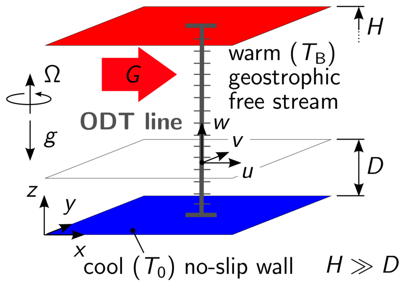
Figure 1 Sketch of the stratified Ekman flow configuration investigated with application of the ODT model. A warm (temperature T_B) geostrophic bulk flow G resides over a rigid surface relative to a corotating frame of reference. The vectors of the angular velocity Ω and gravity g are parallel. A sudden drop of the surface temperature from T_B to T₀ at t=0 is used to prescribe stratification to the Boussinesq fluid due to which the statistically stationary Ekman flow becomes transient. The height H of the columnar ODT domain reaches up into the geostrophic free stream so that the Ekman boundary layer thickness fulfills D≪H and thus acts as reservoir for heat and momentum so that the flow evolves under almost constant bulk–surface temperature difference $\mathrm{\Delta }T=T_{\mathrm{B}}-T_{\mathrm{0}}>\mathrm{0}$.

The initially neutral Ekman flow is fully developed and reaches an approximately statistically stationary state. The initial condition exhibits thermal equilibrium $T=T_{\mathrm{B}}=\mathrm{const}$ for t<0, but not for t ⩾ 0. At t=0, a smooth monotonic temperature profile, which is confined to the viscous surface layer, is prescribed to the turbulent flow and parameterized as

$$\begin{array}{}\text{(1)}& T(z,\mathrm{0})=T_{\mathrm{0}}+\mathrm{\Delta }T\mathrm{erf}\left({\displaystyle \frac{z/D}{\mathrm{2}a}}\right)\end{array}$$

where T₀ is the reference temperature at the surface (z=0) after onset of cooling and $\mathrm{\Delta }T=T_{\mathrm{B}}-T_{\mathrm{0}}$ denotes the prescribed bulk-surface temperature difference, in which the bulk temperature T_B is approached with increasing vertical distance from the surface. Analogous to Ansorge and Mellado (2014), we select the stretching parameter $a=\mathrm{0.15}\ll \mathrm{1}$ in order to confine the smooth initial temperature drop to the viscous surface layer (sublayer). The latter covers only a fraction of the laminar Ekman boundary layer thickness $D=\sqrt{\mathrm{2}\mathit{\nu }/f}$, where f=2Ω is the Coriolis parameter and Ω the prescribed angular velocity of the co-rotating frame of reference.

The steady laminar solution can be analytically obtained by solving the Navier-Stokes or ODT equations under absence of turbulence for the non-zero horizontal velocity components. This solution is given by e.g., Pedlosky (1979)

$$\begin{array}{}\text{(2)}& {\displaystyle }{U}_{\text{lam}}\left(z\right)=G\left[\mathrm{1}-\cos (z/D)e^{-z/D}\right],\text{(3)}& {\displaystyle }{V}_{\text{lam}}\left(z\right)=G\sin (z/D)e^{-z/D},\end{array}$$

where U_lam(z) and V_lam(z) take the form of exponentially damped spatial oscillations with wave length D. D is the Ekman length scale (laminar Ekman layer thickness) that separates the roots of the spatial oscillations in the velocity profiles U_lam(z) and V_lam(z). The bulk flow dissipates its energy over the Ekman timescale $(H/D)/f$ under laminar and $(H/{\mathit{\delta }}_{*})/f$ under turbulent conditions for a fluid layer of height H (e.g., Pedlosky, 1979). Here, $H/D>H/{\mathit{\delta }}_{*}\gg \mathrm{1}$ so that the decay will only be experienced over several hundred inertial periods. Here, only up to 20 inertial periods have been simulated from which 2–5 inertial periods have been used for comparison with reference data.

Based on the selected case set-up and the governing equations, stratified Ekman flow cases are described by the following nondimensional control parameters,

$$\begin{array}{}\text{(4)}& {\displaystyle }\mathit{Pr}={\displaystyle \frac{\mathit{\nu }}{\mathit{\kappa }}}=\mathrm{1},\text{(5)}& {\displaystyle }\mathit{Re}={\displaystyle \frac{GD}{\mathit{\nu }}},\text{(6)}& {\displaystyle }\mathit{Fr}={\displaystyle \frac{G^{\mathrm{2}}}{gD\mathit{\beta }\mathrm{\Delta }T}},\text{(7)}& {\displaystyle }{\mathit{Ri}}_{\mathrm{B}}={\displaystyle \frac{\mathrm{1}}{Fr}}{\displaystyle \frac{{\mathit{\delta }}_{*,\mathrm{0}}}{D}},\end{array}$$

where Pr denotes the Prandtl, Re the Reynolds, Fr the Froude, and Ri_B the bulk Richardson number. Pr is a fluid property that expresses the ratio of the kinematic viscosity ν and the thermal diffusivity κ. For air, Pr≈0.7, which we idealize to Pr=1 in order to facilitate one-to-one comparisons with reference DNS from Ansorge and Mellado (2014). Re expresses the ratio of inertial and viscous forces based on the geostrophically balanced free-stream velocity G, which is assumed to be brought to rest across the laminar Ekman layer thickness D. Likewise, Re may be viewed as an inverse Ekman or Rossby number when interpreted as balance of viscous and Coriolis or inertial and Coriolis forces, respectively. The latter may be more relevant for weakly nonlinear flow regimes (e.g. Ghasemi et al., 2018) but this is less relevant here as we are interested in flow regimes dominated by turbulence. Next, Fr expresses the balance of buoyancy and pressure gradient forces in units of the geostrophic pressure gradient force. Fr is prescribed by application of Eq. (1). In the expression for Fr, g>0 denotes the magnitude of the gravitational acceleration on Earth's surface and $\mathit{\beta }=T_{\mathrm{0}}^{-\mathrm{1}}$ is the thermal expansion coefficient of the assumed ideal gas at reference temperature T₀ in the Oberbeck-Boussinesq limit of small temperature and density variations that are proportional to the buoyancy forces. The length scale ${\mathit{\delta }}_{*,\mathrm{0}}$ denotes the turbulent Ekman boundary layer thickness under neutral conditions at the onset time t=0 of the cooling event. The Ekman length scale D is, in general, not a good estimator for ${\mathit{\delta }}_{*,\mathrm{0}}$ (see, e.g., Ansorge and Mellado, 2014, and the discussion below) so that Ri_B parameterizes the case set-up in terms of the prescribed surface–bulk temperature difference assumed to be present across the turbulent boundary layer for sufficiently short time scales after the surface cooling was established. In the long run, the temperature will not only drop across the turbulent boundary layer but will also extend into the lower part of the bulk. The a priori unknown development of the bulk stratification prevents Ri_B from acting as similarity parameter of the transient flow solution.

3 Modeling approach

This section gives a brief overview of the stochastic ODT model and its application to stratified Ekman flow. The general model set-up and details on the treatment of the Coriolis forces is given in Kerstein and Wunsch (2006), whereas the buoyancy treatment follows Gonzalez-Juez et al. (2013). The physical motivation and mathematical background of the modeling approach is elaborated in Kerstein (1999); Kerstein et al. (2001); Kerstein (2022). Technical details on the fully adaptive finite-volume implementation used in the present study are collected in Lignell et al. (2013); Stephens and Lignell (2021).

3.1 Overview of the ODT model

The one-dimensional turbulence (ODT) model (Kerstein, 1999) is a self-contained dimensionally reduced turbulence model that aims to resolve all relevant scales of a turbulent flow but only in one dimension. The ODT domain is a notional line-of-sight along which synthetic but statistically representative flow profiles are evolved in time. The model distinguishes deterministic molecular-diffusive mixing (which smoothens property gradients by irreversible, dissipative processes) from notionally random turbulent stirring (which increases property gradients) as sketched in Fig. 2. The continuous deterministic evolution of flow profiles is punctuated by discrete eddy events that are stochastically sampled with respect to eddy size ℓ, location z_e, and time of occurrence t_e. Eddy events model the effects of 3-D turbulent advection for the 1-D computational domain. A stochastically sampled ensemble of eddy events during in a flow realization (numerical simulation) replicates cascade phenomenology of Navier–Stokes turbulence. Distribution functions for the three random variables mentioned change with time based on the evolving flow state which is the basis for the model's dynamical complexity.

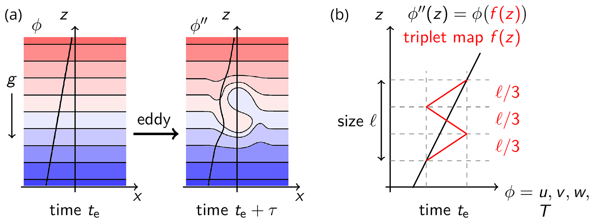
Figure 2 (a) Schematic of an eddy turnover illustrated for an initially linear property profile ϕ(z), where ϕ stands representative for u, v, w, and T. The initial flow state at time t=t_e is denoted as ϕ(z), and the final state at $t=t_e+\mathit{\tau }$ by ϕ^′′(z), where τ is the eddy turnover time. (b) Visualization of the triplet map f(z) that models the microstructure of turbulent “eddies” and is used to formulate the discrete ODT “eddy” events. Eddy events are defined by the random variables location z_e, size ℓ, and occurrence time t_e. Stochastically sampled eddy events punctuate the deterministic flow evolution at times t_e and are sampled with a local rate that depends on the momentary flow state.

ODT has been applied to various types of flows ranging from free-shear flows and jets (e.g., Kerstein et al., 2001; Klein et al., 2019), stable (e.g., Kerstein and Wunsch, 2006) and multiphysical boundary layers (e.g., Monson et al., 2016; Medina M. et al., 2019), to convectively unstable flows (e.g., Wunsch and Kerstein, 2005; Chandrakar et al., 2020), and even canopy roughness effects (Freire and Chamecki, 2018). A comprehensive analysis of the momentum and scalar transfer in canonical boundary-layer-type flows has recently been performed by Fragner and Schmidt (2017); Rakhi et al. (2019); Klein et al. (2022) demonstrating reasonable predictive capabilities across turbulent flow regimes. This renders ODT an interesting candidate for next generation wall models to be utilized preferentially in large-eddy simulation of atmospheric boundary layers (e.g., Freire and Chamecki, 2021; Freire, 2022). Such applications, however, benefit from a comprehensive understanding of the stand-alone model's capabilities and limitations with respect to Ekman flow. Elucidating this further is one goal of the present study.

3.2 ODT conservation equations with stochastic turbulence modeling

For the flow configuration sketched in Fig. 1, the ODT domain is a single line that is aligned with the vertical (z) coordinate. The flow and transport processes are resolved along this line such that the stand-alone model application constitutes a single-column model for atmospheric boundary-layer flows.

The governing equations are the conservation equations of mass, momentum, and energy plus an equation of state. Here we make use of the Oberbeck–Boussinesq approximation with a linear equation of state, $\mathit{\rho }\left(T\right)={\mathit{\rho }}_{\mathrm{r}}[\mathrm{1}-\mathit{\beta }(T-T_{\mathrm{r}}\left)\right]$, where ρ(T) denotes the weakly fluctuating mass density, β the thermal expansion coefficient, and the subscript “r” the reference values. The mass density is taken as a constant except for the buoyancy forces, which yields the governing equations as

$$\begin{array}{}\text{(8)}& {\displaystyle }\begin{array}{rl}{\displaystyle \frac{\partial u_i}{\partial t}}+\sum _{t_e}{\mathcal{E}}_i(u,v,w,T)\stackrel{\mathrm{̃}}{\mathit{\delta }}(t-t_e)& =\mathit{\nu }{\displaystyle \frac{{\partial }^{\mathrm{2}}{u}_i}{\partial z^{\mathrm{2}}}}\\ & -f{\mathit{ϵ}}_{i\mathrm{3}k}\left(u_k-G{\mathit{\delta }}_{k\mathrm{1}}\right),\end{array}\text{(9)}& {\displaystyle \frac{\partial T}{\partial t}}+\sum _{t_e}{\mathcal{E}}_T(u,v,w,T)\stackrel{\mathrm{̃}}{\mathit{\delta }}(t-t_e)=\mathit{\kappa }{\displaystyle \frac{{\partial }^{\mathrm{2}}T}{\partial z^{\mathrm{2}}}},\end{array}$$

where z denotes the vertical (wall-normal) coordinate, t the time, $\left(u_i\right)=(u,v,w{)}^T$ with $i\in \mathit{\{}\mathrm{1},\mathrm{2},\mathrm{3}\mathit{\}}$ the velocity vector components with respect to the Cartesian coordinates $(x,y,z)$, T the temperature, ν the kinematic viscosity and κ the thermal diffusivity of the fluid, f=2Ω the inertial frequency due to model-resolved horizontal Coriolis forces, Ω the vertical component of the system's angular velocity, G the geostrophically balanced bulk flow velocity, δ_ij the Kronecker symbol, and ϵ_ijk the Levi–Civita tensor. Einstein's summation convention is implied. The second term on the left-hand side of Eqs. (8) and (9) is a symbolic representation of turbulent eddies that are modeled by a stochastically sampled sequence of mapping events ℰ that modify property profiles by instantaneous application of the triplet map f(z) as sketched in Fig. 2. Eddy events occur at discrete times t_e. Eddy events obey physical conservation principles by utilizing measure-preserving mapping operations. The sum over a sequence of Dirac $\stackrel{\mathrm{̃}}{\mathit{\delta }}$ functions indicates the instantaneous nature of the eddy events.

A sequence of ODT eddy events aims to reproduce the statistical properties and variability of the corresponding turbulent flow. As a result of the oversampling and rejection algorithm summarized above, eddy events are implemented at a local time-varying rate governed by the frequency

$$\begin{array}{}\text{(10)}& {\mathit{\tau }}^{-\mathrm{1}}\simeq C\sqrt{{\displaystyle \frac{\mathrm{1}}{{\mathrm{\ell }}^{\mathrm{2}}}}\sum _{i=\mathrm{1}}^{\mathrm{3}}{u}_{i,K}^{\mathrm{2}}+{\displaystyle \frac{\mathrm{8}}{\mathrm{27}\mathrm{\ell }}}g\mathit{\beta }{T}_K-Z{\displaystyle \frac{{\mathit{\nu }}^{\mathrm{2}}}{{\mathrm{\ell }}^{\mathrm{4}}}}},\end{array}$$

which is positive for a real-valued square root and zero otherwise. The three terms under the square root represent the current eddy-available specific kinetic energy, the specific gravitational potential energy, and the specific viscous penalty energy, respectively. The first two terms are obtained from the mapping kernel $K\left(z\right)=z-f\left(z\right)$ weighted velocity u_i,K and Boussinesq temperature T_K that are detailed in Gonzalez-Juez et al. (2013). Furthermore, ℓ denotes the selected eddy size, and C and Z are the adjustable ODT eddy-rate and viscous penalty parameters. Eq. (10) is the basis for the physically based turbulence modeling in ODT. Finite velocity shear is needed in order to drive turbulence under stable and neutral conditions, whereas turbulence may be driven spontaneously under unstable conditions with the fluid at rest. In both cases, viscous damping effects (formulated as specific viscous penalty energy) need to be overcome to yield a finite eddy frequency.

Equation (10) is applicable only if the eddy-available energy is positive because negative eddy-available energy implies an energetically forbidden eddy. For turbulence in stably stratified flow, this constraint is related to a local interpretation of the $\mathrm{1}/\mathrm{4}$ criterion for self-sustained turbulence (Miles, 1961; Howard, 1961). This was discussed previously by Wunsch and Kerstein (2001). ODT eddy events are energetically permitted when the local gradient Richardson number fulfills

$$\begin{array}{}\text{(11)}& R{i}_{\mathrm{g}}={\displaystyle \frac{g\mathit{\beta }\frac{\partial T}{\partial z}}{{\left(\frac{\partial u_{\text{h}}}{\partial z}\right)}^{\mathrm{2}}}}\lesssim \mathrm{0.25},\end{array}$$

which gives the ratio of the turbulence suppressing stratification in terms of $\partial T/\partial z$ and the turbulence generating vertical velocity shear $\partial u_{\text{h}}/\partial z$, where $u_{\text{h}}=\sqrt{u^{\mathrm{2}}+v^{\mathrm{2}}}$ denotes the horizontal flow velocity. Assuming linear profiles u(z)∼az and T(z)∼bz for $v\left(z\right)=w\left(z\right)=\mathrm{0}$ without loss of generality and neglecting the viscous penalty by selecting Z=0, the condition Ri_g=0.25 is obtained from Eq. (10) for the marginal eddy as shown by Gonzalez-Juez et al. (2011a). While this aspect suggests consistence with established theory, the original derivation of the $\mathrm{1}/\mathrm{4}$ criterion considers the ensemble-averaged state, whereas in the ODT realizations, like in reality, flow profiles fluctuate. Instantaneous property profiles are in fact never linear and often not even monotonic (see momentary T(z) in Fig. 8c below). This suggests that Ri_g of the ensemble-averaged state may reach significantly larger values than $\mathrm{1}/\mathrm{4}$ while turbulence is still observed. In such cases, Ri_g may locally but momentarily yield values smaller than $\mathrm{1}/\mathrm{4}$ for a certain size range of eddies. Hence, violation of the $\mathrm{1}/\mathrm{4}$ criterion for the ensemble-averaged state does neither contradict evidence from observations (e.g., Galperin et al., 2007; Zilitinkevich et al., 2013) nor ODT model predictions. The latter are discussed in more detail below.

4  Model calibration for neutral conditions

In the following, the adjustable model parameters C and Z are calibrated for neutral Ekman flow that is characterized by Fr→∞ and Ri_B=0. First, we select model parameters based on the Re dependence of the bulk quantities friction velocity and surface wind-turning angle. After that, the velocity boundary layer and the budget balance of the turbulence kinetic energy are analyzed.

4.1 Surface drag law

The ODT model parameters C and Z introduced above need to be calibrated for Ekman flows since Coriolis forces may break previous model calibrations for nonrotating flow. The calibration procedure has been explained for channel (e.g., Schmidt et al., 2003) and plate boundary layer flows (e.g., Fragner and Schmidt, 2017; Rakhi et al., 2019), among other cases, so that we do not repeat this here. Instead, we test the sensitivity of bulk quantities for three preselected sets of model parameters under neutral conditions which is justified next.

For the stable atmospheric boundary layer, Kerstein and Wunsch (2006) used C=5.9 and Z=0 for a case set-up of the GABLS model intercomparison (Cuxart et al., 2006). These model parameter values are close to our present calibration albeit there are differences in the model application with respect to the resolved range of scales. Kerstein and Wunsch (2006) applied ODT in “LES mode”, where ODT is used to extend the resolved range of inertial scales without reaching the viscous scales. The unresolved turbulence was modeled by a conventional turbulent eddy viscosity approach. In this set-up, all eddy sizes above the grid cell size are physically relevant such that the small-scale suppression parameter was set to Z=0. This implies that stochastic sampling is performed with a finite rate down to the grid resolution.

In the present study, ODT is used in “DNS mode” in which all relevant flow scales, down to the viscous scales, are resolved along a 1-D physical coordinate. Viscous suppression, hence, bounds the physically meaningful turbulence scales from below based on energetic considerations. For Z>0 in Eq. (10), ODT eddy events are suppressed by the specific viscous penalty energy. Note that Z=1 means preferential suppression of eddy events below the viscous length scale, but larger turbulent scales might also be significantly affected because the viscous penalty, albeit size dependent, reduces the available energy of eddies of all sizes. Here we utilize the expression for the viscous penalty proposed by Kerstein (1999), but implemented on an adaptive grid (Lignell et al., 2013).

Eddy events are randomly sampled by oversampling of candidate eddies followed by a rejection step in which the eddy acceptance probability is evaluated using Eq. (10) (Gonzalez-Juez et al., 2013). In addition, the “two-thirds” method (e.g., Fragner and Schmidt, 2017; Rakhi et al., 2019) is applied requiring positive net available energy in two out of three segments of the triplet map in order to suppress unphysical growth of the boundary layer for the present neutral and transient stable configurations.

We note that Kerstein and Wunsch (2006) did not use the “two-thirds” method since their overall stable stratification sufficed to suppress unphysically large eddy events. This is because stable stratification yields a positive specific potential energy in Eq. (10) that acts analogously to the specific viscous penalty energy.

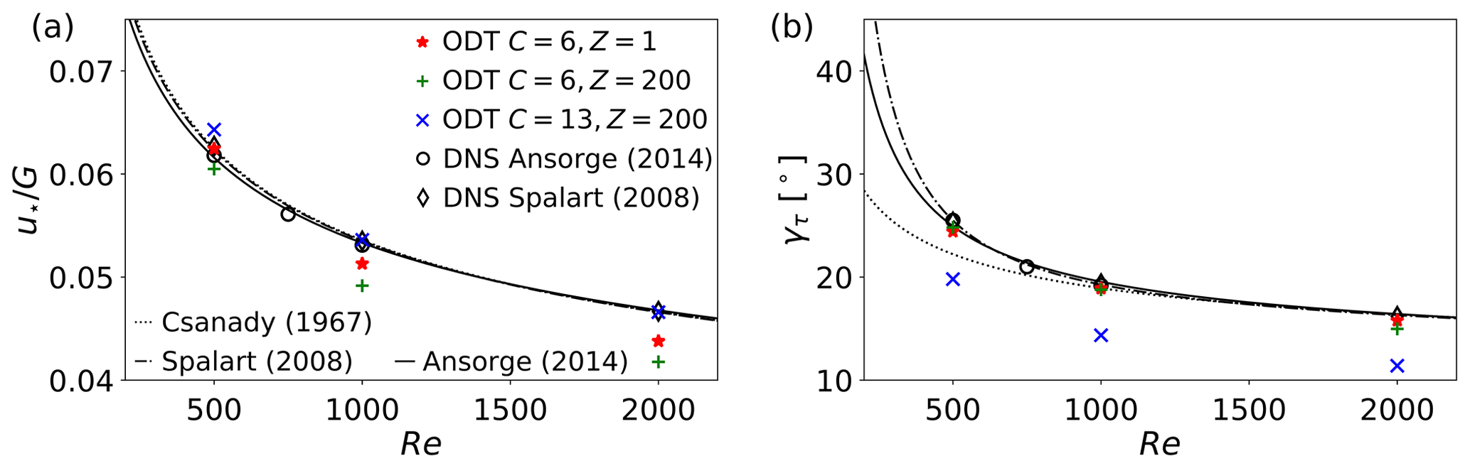
Figure 3 (a) Normalized friction velocity $u_{*}/G$ and (b) surface wind-turning (wall-shear) angle γ_τ as function of Re for various sets of ODT model parameters (filled symbols) in comparison to reference DNS (open symbols) and theory (lines) compiled from Csanady (1967); Spalart et al. (2008); Ansorge and Mellado (2014). See the text and Table 1 for details.

Csanady (1967)Spalart et al. (2008)Ansorge and Mellado (2014)

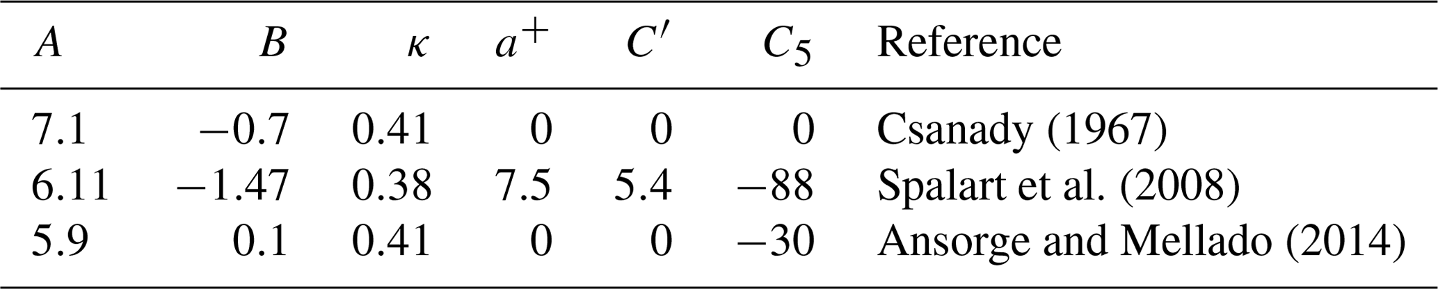
Table 1 Parameterization coefficients for the turbulent drag over a smooth surface.

The surface drag law denotes the Re dependence of the friction velocity u_* and the surface wind-turning (wall-shear) angle γ_τ as described by Eqs. (14)–(17).

Next, we present the case of neutral Ekman flow for the purpose of model calibration. Figure 3 shows the friction velocity u_* and the corresponding wall-shear angle γ_τ (wind-turning angle measured at the surface z=0) as function of Re for ODT, reference DNS, and theory. The friction velocity and wall-shear angle are defined based on the temporal-averaged horizontal velocity components, U(z) and V(z), as

$$\begin{array}{}\text{(12)}& {\displaystyle }{u}_{*}=\sqrt{\mathit{\nu }{\displaystyle \frac{\text{d}\sqrt{U^{\mathrm{2}}+V^{\mathrm{2}}}}{\text{d}z}}{|}_{z=\mathrm{0}}},\text{(13)}& {\displaystyle }{\mathit{\gamma }}_{\mathit{\tau }}=\arctan \left({\left.{\displaystyle \frac{\text{d}V/\text{d}z}{\text{d}U/\text{d}z}}\right|}_{z=\mathrm{0}}\right).\end{array}$$

Note that the neutral Ekman flow reaches an almost statistically stationary state such that temporal flow statistics can be gathered analogously to the available reference DNS. The driving geostrophic bulk flow slowly dissipates its kinetic energy on the Ekman time scale $(H/D)f^{-\mathrm{1}}$ (e.g., Pedlosky, 1979), or rather, $(H/{\mathit{\delta }}_{*,\mathrm{0}})f^{-\mathrm{1}}$ under turbulent conditions, which is much longer than the simulated time since $H\gg {\mathit{\delta }}_{*,\mathrm{0}}>D$.

For a smooth surface, reference values of u_* and γ_τ may be obtained for arbitrary Re with the aid of the generalized similarity theory of Spalart et al. (2008). This theory yields u_* and γ_τ by the following parameterization (see Spalart et al., 2008, but let their $-\mathcal{A}=\mathit{\kappa }B$ and ℬ=κA in accordance with Coleman et al., 1990)

$$\begin{array}{}\text{(14)}& {\displaystyle \frac{G}{u_{*}}}\cos \mathit{\theta }-{\displaystyle \frac{\mathrm{1}}{\mathit{\kappa }}}\ln \left({\displaystyle \frac{u_{*}^{\mathrm{2}}}{f\mathit{\nu }}}+a^{+}\right)=B,\text{(15)}& {\displaystyle \frac{G}{u_{*}}}\sin \mathit{\theta }=A,\end{array}$$

in which

$$\begin{array}{}\text{(16)}& {\displaystyle }\mathit{\theta }={\mathit{\gamma }}_{\mathit{\tau }}+{\displaystyle \frac{f\mathit{\nu }}{u_{*}^{\mathrm{2}}}}\left[C_{\mathrm{5}}-{\displaystyle \frac{a^{+}}{\mathit{\kappa }}}\left(\ln \left({\displaystyle \frac{a^{+}f\mathit{\nu }}{u_{*}^{\mathrm{2}}}}\right)+C^{\prime }\mathit{\kappa }-\mathrm{1}\right)\right],\text{(17)}& {\displaystyle }{\mathit{Re}}_{\mathit{\tau }}={\displaystyle \frac{u_{*}^{\mathrm{2}}}{f\mathit{\nu }}}={\displaystyle \frac{R{e}^{\mathrm{2}}}{\mathrm{2}(G/u_{*}{)}^{\mathrm{2}}}},\end{array}$$

where θ denotes the modified wall-shear angle, κ the von Kármán constant, Re_τ the friction Reynolds number, and A, B, C^′, C₅, and a⁺ numerical parameterization constants. Some common parameter values are given in Table 1 with the corresponding Re dependence shown in Fig. 3. The angle γ_τ exhibits a larger uncertainty for Re ≲ 1000 than the friction velocity u_*, which is reasonably reproduced by all parameterizations.

To summarize, model predictions shown in Fig. 3 exhibit reasonable agreement with the reference data demonstrating that it is possible to calibrate the ODT model such that either the friction velocity (C=13, Z=200) or the wall-shear angle (C=6, Z=1) is reproduced for arbitrary Re. A correct representation of the wall-shear angle is deemed favorable as it suggests reasonable representation of relevant properties of Ekman flow turbulence (e.g., Lüpkes and Schlünzen, 1996; Zilitinkevich et al., 1999). Model parameter values C=6 and Z=200 are close to a high-Re calibration for channel flow (Klein et al., 2022), but they are not optimal for Ekman boundary layers, neither at small nor large Reynolds number. Based on the results shown in Fig. 3, we select C=6 and Z=200 for small Re=500, but Z=1 for moderately high Re=1000 and 2000 investigated. Details of these calibrated ODT set-ups are summarized in Table 2. Snapshots from the neutral case simulations are used to generate ensembles of turbulent initial conditions for the stratified cases as described below.

Table 2 Details of the ODT simulation cases for neutral Ekman flow with comparison to reference DNS.

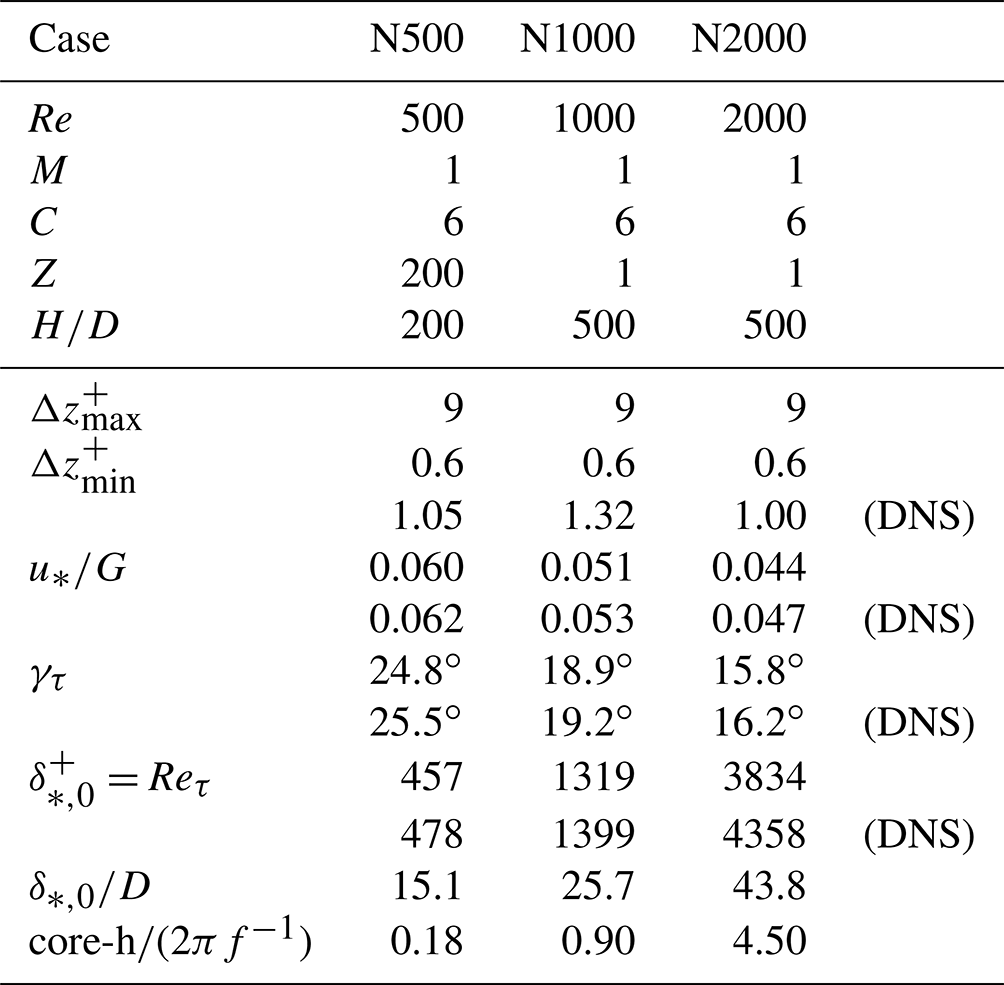
Inputs that characterize the ODT case set-up are given above the middle line. Outputs that characterize the flow state are given below the middle line for ODT and corresponding reference DNS for Re=500, 1000 (Ansorge and Mellado, 2014), and 2000 (Spalart et al., 2008). Core hours (core-h) spent per inertial period (2πf⁻¹) were measured on an Intel^® Xeon^® E5-2630 (2.40 GHz) processor. Only a single flow realization (M=1) is run in order to obtain temporal flow statistics.

4.2 Velocity boundary layer

With the model calibrations at hand, we proceed by analyzing the boundary layer structure for neutral conditions. This is important because the fully developed neutral flow will be used below as initial condition for the stratified cases.

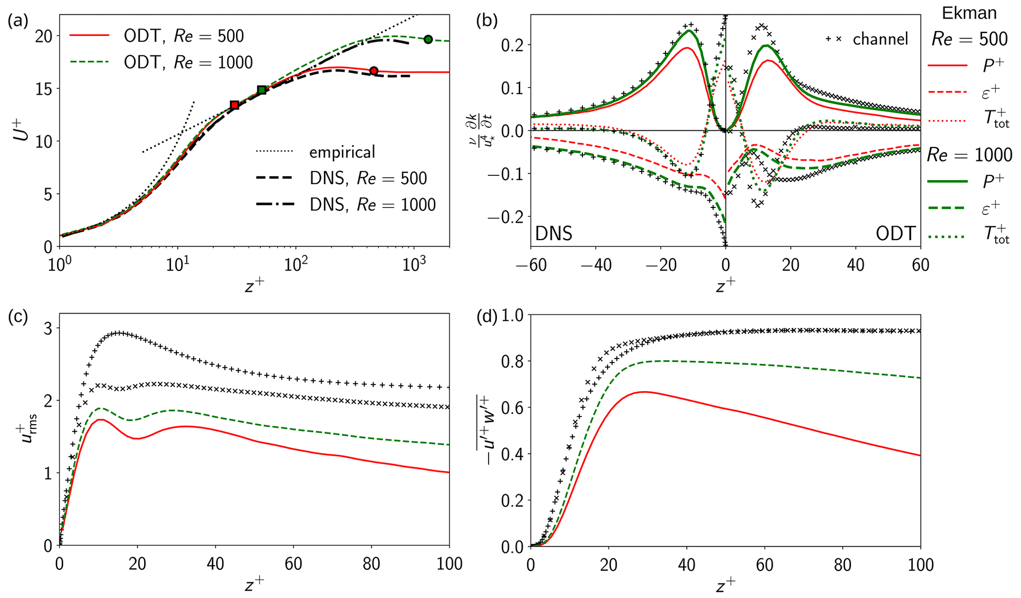
Figure 4 (a) Law-of-the-wall plot of the normalized temporal-averaged geostrophic (streamwise) velocity $U^{+}=U/u_{*}$ over the stretched vertical coordinate $z^{+}=z{u}_{*}/\mathit{\nu }$. Empirical relations are given for the viscous sublayer close to the surface and the log layer at finite distance from the surface according to Eqs. (18) and (19). Symbols mark the locations corresponding to the laminar Ekman layer thickness $z^{+}=D^{+}$ (□) and the turbulent Ekman layer thickness $z^{+}={\mathit{\delta }}_{*,\mathrm{0}}^{+}$ (∘), respectively. ODT simulation results have been obtained for the cases N500 (thin lines) and N1000 (thick lines) detailed in Table 2. Colors encode the model parameter selections in accordance with Fig. 3. Corresponding reference DNS are from Ansorge and Mellado (2014). (b) “Back-to-back plot” of the turbulence kinetic energy (TKE) budget for fully developed Ekman flow under neutral conditions in comparison to reference DNS (Lee and Moser, 2015) and ODT (Klein et al., 2022) results for turbulent channel flow for Re_τ=2000. (c) Normalized streamwise fluctuation velocity $u_{\text{rms}}^{+}$ and (d) eddy covariance $\stackrel{\mathrm{‾}}{{u^{\prime }}^{+}{w^{\prime }}^{+}}$ for ODT Ekman flow (lines) in comparison to ODT (×) and DNS (+) channel flow.

Figure 4a shows simulated profiles of the normalized temporal-averaged geostrophic (streamwise) velocity component $U^{+}=U/u_{*}$ as function of the stretched boundary-layer coordinate $z^{+}=z{u}_{*}/\mathit{\nu }$. ODT results for the Re-dependent selection of the model parameter Z are shown together with reference DNS from Ansorge and Mellado (2014). The model is capable of satisfactorily reproducing the reference DNS. Some profile variability can be discerned that are unrelated to the friction velocity and wall-shear angle, which are both rather well reproduced for the low Reynolds numbers investigated here. However, ODT underestimates the boundary layer thickness ${\mathit{\delta }}_{*,\mathrm{0}}$ in comparison to the available reference DNS so the that predicted normalized velocity U⁺ tends to be higher than the reference data towards the bulk, but the effect is weak. Nevertheless, all simulated profiles exhibit the law of the wall that consists of the linear viscous surface layer,

$$\begin{array}{}\text{(18)}& U^{+}\left(z^{+}\right)=z^{+}\text{for}{z}^{+}\lesssim \mathrm{5},\end{array}$$

and the log layer,

$$\begin{array}{}\text{(19)}& U^{+}\left(z^{+}\right)={\displaystyle \frac{\mathrm{1}}{\mathit{\kappa }}}\ln z^{+}+B^{\prime }\text{for}\mathrm{30}\lesssim z^{+}\lesssim \mathrm{0.1}{\mathit{\delta }}_{*,\mathrm{0}}^{+},\end{array}$$

where ${\mathit{\delta }}_{*,\mathrm{0}}$ and κ were introduced above but the additive constant B^′ differs from previous coefficients. The given z⁺ range follows convention (e.g., Pope, 2000) and only serves approximate descriptive purposes skipping any elaboration on meso layers and scaling modifications. Here, κ=0.41 and $B^{\prime }=\mathrm{5.0}$ have been selected for comparison (e.g., Ansorge and Mellado, 2014). It is worth noting that ODT captures the jet in the outer layer which is located at $z^{+}⩽O\left({\mathit{\delta }}_{*,\mathrm{0}}^{+}\right)$. This jet has shape and magnitude comparable to reference data (e.g., Spalart et al., 2008; Ansorge and Mellado, 2014; Maronga and Li, 2022; Liu et al., 2021a, not shown here). This demonstrates the self-similar boundary-layer structure with respect to inner and outer layer similarity.

Two locations corresponding to layer heights (length scales) are marked by symbols and are given for orientation. One is the turbulent boundary layer thickness ${\mathit{\delta }}_{*,\mathrm{0}}$, which is located above the maximum of the low-level jet. The second is the laminar Ekman boundary layer thickness D, for which the averaged cross-isobaric flow component V reaches its maximum. Details of the associated wind turning effects are further discussed below. Note that for Re=500, D is still in the buffer layer since $D^{+}\approx \mathrm{30}$. By contrast, for Re=1000, $D^{+}\approx \mathrm{60}$ is found at the lower end of the log layer, which is properly realized only for $z^{+}\gtrsim \mathrm{100}$. The different numerical values of D⁺ together with the physical implications of boundary layer similarity (law of the wall) at least partly explains the model parameter dependence on Re that was noted above.

For completeness, but without detailed discussion, Figs. 4c and d show boundary layer profiles of the streamwise (geostrophic) fluctuation velocity, $u_{\mathrm{rms}}=\sqrt{\stackrel{\mathrm{‾}}{u^{\mathrm{2}}}-U^{\mathrm{2}}}$, and the eddy covariance, $\stackrel{\mathrm{‾}}{u^{\prime }{w}^{\prime }}$, of the geostrophic and vertical velocity fluctuations, respectively. The ODT results are shown together with corresponding ODT (Klein et al., 2022) and DNS (Lee and Moser, 2015) results for pressure-driven turbulent channel flow. ODT exhibits a known modeling error that manifests itself by an unphysical lack in fluctuation magnitude across the boundary layer (see Lignell et al., 2013). Because the map-based representation of turbulent fluxes is decoupled from the fluctuation variance, the model is able to reasonably capture the near-surface turbulent fluxes as demonstrated by the channel flow data (see Klein et al., 2022). Note that Ekman flow statistics approach those from channel flow with increasing Re suggesting applicability of inner-layer similarity for high asymptotic Reynolds numbers among different case set-ups.

4.3 Turbulence kinetic energy budget

We proceed by assuming statistically stationary Ekman flow and analyze the turbulent fluctuations resolved by the model. Further insight into the dynamics is given by the turbulence kinetic energy (TKE) budget, which is discussed next. Figure 4b shows the following normalized model-resolved contributions to the TKE budget

$$\begin{array}{}\text{(20)}& \mathrm{0}=P^{+}+T_{\mathrm{tot}}^{+}+{\mathit{\epsilon }}^{+},\end{array}$$

in which P denotes the production, T_tot the total transport, and ε the dissipation of temporal-averaged turbulence kinetic energy $k=\frac{\mathrm{1}}{\mathrm{2}}\stackrel{\mathrm{‾}}{u_i^{\prime }{u}_i^{\prime }}$. Normalization of these terms was performed by division with $u_{*}^{\mathrm{4}}/\mathit{\nu }$. The model resolved dimensional expressions of the contributions are given by

$$\begin{array}{}\text{(21)}& {\displaystyle }P=-\stackrel{\mathrm{‾}}{u^{\prime }{w}^{\prime }}{\displaystyle \frac{\text{d}U}{\text{d}z}}-\stackrel{\mathrm{‾}}{v^{\prime }{w}^{\prime }}{\displaystyle \frac{\text{d}V}{\text{d}z}},\text{(22)}& {\displaystyle }\mathit{\epsilon }=-\mathit{\nu }\stackrel{\mathrm{‾}}{{\displaystyle \frac{\partial u_i^{\prime }}{\partial z}}{\displaystyle \frac{\partial u_i^{\prime }}{\partial z}}},\text{(23)}& {\displaystyle }{T}_{\mathrm{tot}}=-{\displaystyle \frac{\text{d}\stackrel{\mathrm{‾}}{u_i^{\prime }{u}_i^{\prime }{w}^{\prime }}}{\text{d}z}}+\mathit{\nu }{\displaystyle \frac{{\text{d}}^{\mathrm{2}}k}{\text{d}{z}^{\mathrm{2}}}},\end{array}$$

as for canonical boundary layers (Kerstein, 1999) by using a spatially uniform high-resolution statistics grid. A cubic spline interpolation is used to transfer momentary flow profile data from the adaptive to the uniform grid. Statistical moments are obtained by temporal averaging of the developing ODT solution. In addition, conditional statistics are used to obtain the turbulent transport terms $\stackrel{\mathrm{‾}}{u_i^{\prime }{w}^{\prime }}$ and $\stackrel{\mathrm{‾}}{u_i^{\prime }{u}_i^{\prime }{w}^{\prime }}$ from the sequence of eddy-induced profile modifications as described in Gonzalez-Juez et al. (2013) and Klein et al. (2022).

Note that T_tot obtained by ODT has turbulent advective and viscous contributions, but it lacks pressure transport as this is not resolved by ODT. Nevertheless, the resolved terms must sum up to a balance, which is monitored in order to decide when second order statistics have sufficiently converged. The ODT results shown in Fig. 4b demonstrate that the model captures the individual contributions acceptably well, in particular the TKE production and its Re dependence. Less agreement is obtained for the TKE dissipation. This is a known modeling artifact (Kerstein, 1999), which can be attributed to the fixed micro-structure of the triplet map and its repeated application at the wall (Lignell et al., 2013). Due to missing pressure transport and less dissipation, a slightly different budget balance is obtained by ODT in comparison to reference DNS. Especially the transport term $T_{\mathrm{tot}}^{+}$ is notably different from the reference data for $z^{+}\lesssim \mathrm{10}$.

Altogether, the ODT model is able to capture relevant features of the temporal-averaged mean state and the corresponding velocity fluctuations in turbulent Ekman boundary layers under neutral conditions. With the calibrated model set-ups, we move on by investigating how the flow interacts with a prescribed initial stratification profile.

5  Model application to stably stratified Ekman flow

In this section we investigate stratification effects with ODT as stand-alone flow model using ensemble-averaged and instantaneous property profiles for various Re and Fr keeping all other physical and calibrated model parameters fixed.

5.1 Temporal flow evolution

The case set-ups and characterizing bulk quantities are summarized in Table 3. But before we discuss results, we briefly describe how ensemble statistics are obtained for the temporally evolving, stratified cases. For each combination of Re and Fr investigated, an ensemble of M=1000 flow realizations is used to aggregate ensemble data for the transient boundary layer. The M ensemble is formed by recording M snapshots of instantaneous flow profiles from the statistically stationary state of the corresponding neutral Ekman flow case. The relevant information is collected in Table 2. After the turbulent velocity field has been obtained, model restarts with a prescribed stratification are prepared. This is achieved by prescribing the smooth but strongly localized initial temperature profile of Eq. (1) to the adaptive grid of the current snapshot of neutrally stratified flow realization. The next step is running the ensemble of M autonomous ODT realizations in parallel by performing a modified model restart. Simulations are continued for at least 5 inertial periods for comparison with reference data, but we have almost always run them up to 20 inertial periods. Model output is obtained as flow profiles and statistical moments of time-window-based averages centered at predefined points in time and as high-resolution time series of flow variables at predefined locations. Conventional ensemble statistics are applied to the sampled data.

Table 3 Overview of the transient stratified cases simulated with ODT.

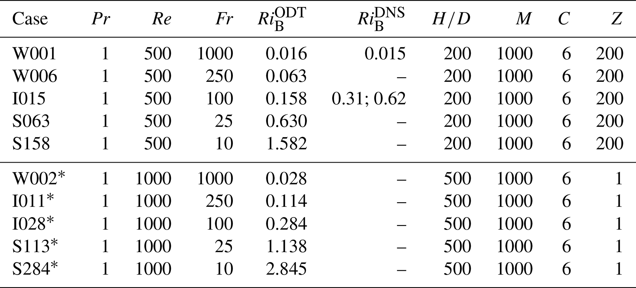
Case prefixes denote weak (W), intermediate (I), and strong (S) stratification regimes. The asterisk (^*) distinguishes Re=500 from 1000. The basic model set-up depends on Re and is adopted from Table 2. M=1000 ensembles were run in parallel on workstations covering up to $t^{-}=\mathrm{20}$ inertial periods for each member. The ODT computational effort for the stable cases is comparable to that of the neutral cases. Ri_B characterizes the flow set-up by the turbulent initial condition and is given for ODT and available Re=500 reference DNS from Ansorge and Mellado (2014). In DNS, different Ri_B have been used but only one in ODT. ODT overestimates the boundary layer thickness so that, for the case I015, Ri_B is smaller than in the DNS.

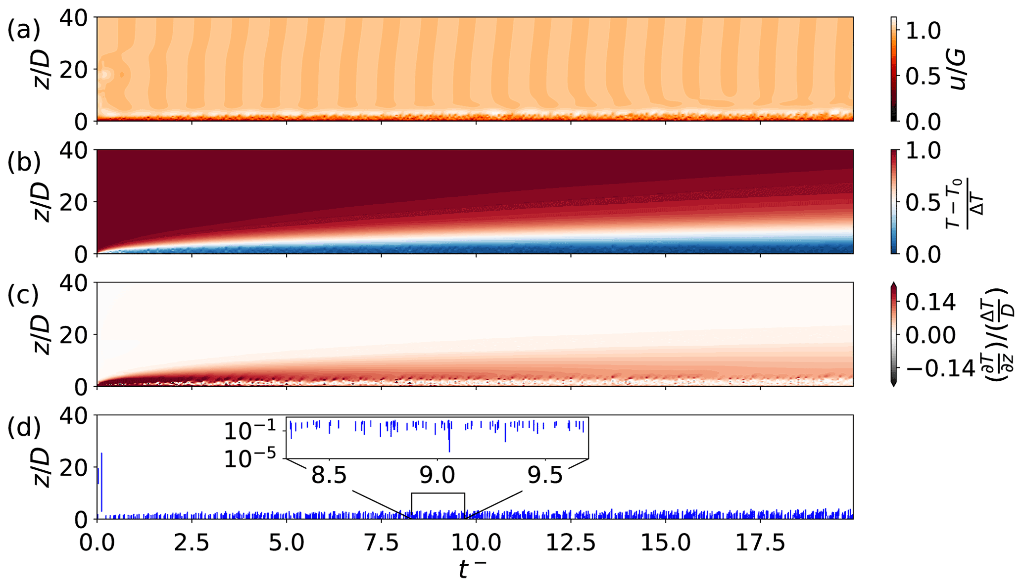
Figures 5 and 6 show the temporal evolution of the stable Ekman boundary layer for various observables simulated with a single ODT realization for the weakly and strongly stratified case W001 and S158, respectively. The simulation results of the stochastic model visually exhibit a statistically steady state in the near-surface region where turbulence is confined for $t^{-}\gtrsim \mathrm{2}$, that is, after an initial transient of about 1–2 inertial periods. Profiles of the momentary temperature T(z,t) and temperature gradient $[\partial T/\partial z](z,t)$ shown in panels (b) and (c), respectively, reveal the structure of the stable boundary layer. Both variables are qualitatively similar to reference LES at much higher Re (Taylor and Sarkar, 2008, Fig. 12) A very thin diffusive surface layer is followed by a shear-driven mixed layer that reduces in size when stratification is increased by decreasing Fr (increasing Ri_B). The temperature inversion is located at about $z/D\approx \mathrm{18}$ in Fig. 5b, c but at a three times lower value $z/D\approx \mathrm{6}$ in Fig. 6b, c for the same case-defining Reynolds number Re. The temperature inversion can be visually identified as the location where the (mean) temperature gradient reaches its maximum. The nonturbulent outer region contains the warm geostrophically balanced bulk flow that acts as a momentum and internal energy reservoir and can be taken as approximately constant for the simulated time interval. The present case set-up is qualitatively comparable, but not identical, to the bottom Ekman layer setup of Taylor and Sarkar (2008, Fig. 3). In contrast to these reference LES, ODT resolves significantly more fine-scale turbulent flow features as it makes high resolution transient numerical simulations feasible. Present ODT simulations were performed for a factor ≈10–20 lower Reynolds numbers than the reference LES demonstrating that the LES contains a significant range of unresolved flow scales that are statistically modeled, which is strictly avoided in the present study.

Next, the profiles of the momentary geostrophic velocity component u(z,t) shown in Figs. 5a and 6a exhibit a near-surface turbulent region but details are hard to see in the present scaling so that we address the boundary layer structure separately below. The turbulent boundary layer thickness visually corresponds with the height of the inversion indicating that velocity or temperature can be used to define the boundary layer thickness (e.g., Seidel et al., 2012) that can be compared with observations or reference simulations if desired.

An interesting dynamical feature is the persistent inertial oscillation that is exhibited by u(z,t) shown in Figs. 5a and 6a. This oscillation manifests itself by periodic modulation (with Coriolis frequency f) of the horizontal velocity components. The oscillation is only observed in the nonturbulent region above the temperature inversion. Even though stand-alone ODT does not resolve inertia–gravity waves, it is remarkable that an inertial oscillation occurs within the dimensionally reduced framework. Qualitatively similar flow features have been observed previously in DNS (Ansorge and Mellado, 2014, 2016, e.g.) and LES (Maronga and Li, 2022, Fig. 1). In the latter, a GABLS case with prescribed surface heat-flux is studied, whereas the former investigates the same set-up as the present ODT study. The inertial oscillations are partly discussed for the reference LES but less for the DNS so that, in the following, we refer to the reference LES for comparison.

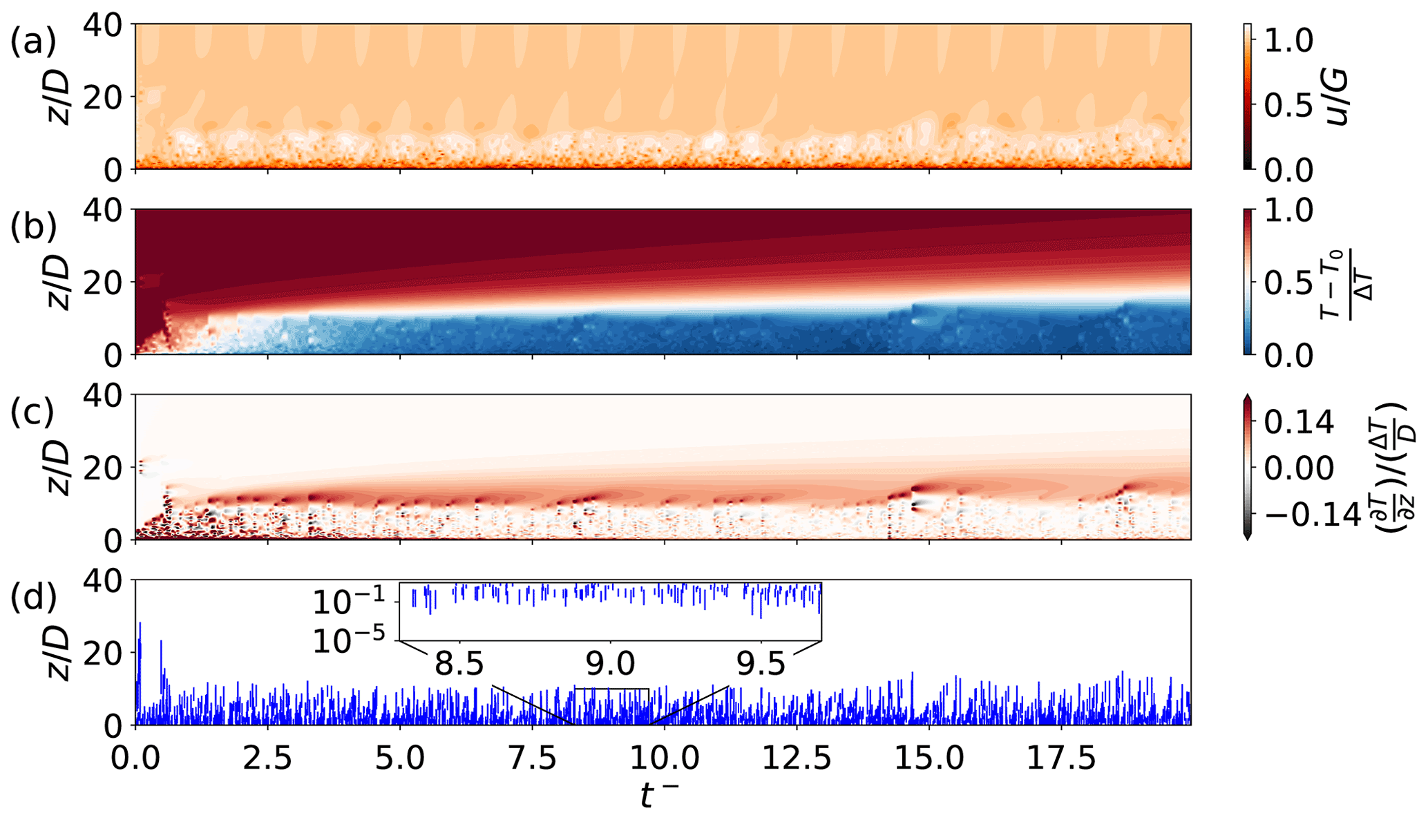
Figure 5 Hovmöller diagrams of various observables showing the temporal evolution of the momentum and thermal boundary layer for a single ODT realization of the weakly stratified case W001 with Re=500 and Fr=1000. (a) Momentary velocity component u(z,t), (b) momentary temperature T(z,t), (c) momentary temperature gradient $[\partial T/\partial z](z,t)$, and (d) sequence of implemented ODT eddy events visualized by instantaneous vertical line intervals. In each plot the vertical coordinate has been truncated for visibility.

Figure 6 Same as Fig. 5 but for case S158 with Re=500 and Fr=10.

The inertial oscillations are oblique in the reference LES from Maronga and Li (2022), where they remain confined to a layer-like region in vertical direction. This might be due to inertial–gravity wave trapping in a laminar stratified layer between the insufficiently stratified bulk and well-mixed surface layer. Also numerical Rayleigh damping utilized at the top of the LES domain might contribute to the vertical truncation of the inertial oscillation. In the present ODT set-up, the inertial oscillation extends into the fluid bulk. This suggests that it is decoupled from the stratification, which is initially zero in the bulk of the fluid as shown in Figs. 5c and 6c. The physical mechanism responsible for the oscillation can only be related to the action of the Coriolis forces that periodically (with frequency f) exhange momentum between the horizontal u (i=1) and v (i=2) velocity components as can be deduced from the lower-order momentum Eq. (8). Stratification effects, within ODT, are only incorporated for the sampling of turbulent eddies. Note that Coriolis–pressure couplings are not resolved by ODT so that inertial oscillations (in the form of inertia gravity waves; see e.g. Pedlosky, 1979) cannot propagate at oblique angles in Figs. 5a or 6a.

In the present ODT application, the forcing is entirely due to the uniform geostrophic bulk flow, but the origin of the inertial oscillation seems to correlate with the onset of the surface cooling at $t^{-}=\mathrm{0}$. It is maintained over long time scales but only for turbulent flow conditions. The oscillation, in fact, decays more rapidly under laminarizing flow conditions obtained by reducing the ODT rate parameter to C=0 which is not shown here since u(z,t) looks qualitatively similar. So the oscillation is caused by the sudden perturbation as in the reference DNS (Ansorge and Mellado, 2014), but present results suggest that it is sustained by a turbulent forcing mechanism. We remind that the ODT equations form a physically damped-driven system, in which damping is due to internal friction (molecular processes) and driving due to geostrophic forcing. Stochastically sampled eddy events only redistribute momentum and energy so that there is no artificial energy input into the system. This constitutes a fundamental difference to other stochastic approaches that are based on the Langevin equation (e.g. Pope, 2000) in which a stochastic process often acts as a source term that may have to be balanced by additional but not always physically justified damping terms. Clarification of the physical mechanism that sustains the inertial oscillation for turbulent flow is therefore an interesting subject that is beyond the scope of this paper and awaits clarification. A possible intermediate step towards a better understanding of the physical processe might be oscillatory Ekman flow. Ashkenazy et al. (2015) provide a lower-order model for ocean currents driven by oscillatory wind shear corresponding to the canonical laboratory experiment described in Vincze et al. (2019). The latter model is based on a Langevin approach with additional linear damping. The model explains some observations but it has been argued that it demands a vertically varying damping coefficient for a more convincing match with observations hinting at physical model limitations. Nevertheless, Ashkenazy's model might serve as a reasonable starting point for an extension to the atmospheric boundary layer. Combining it with the ODT might allow to get rid of the artificial damping term in order to find a physically more consistent lower-order representation of multi-physics geophysical boundary layer flows.

Last, Figs. 5d and 6d show implemented sequences of ODT eddy events for a single ODT flow realization. ODT eddy events are applied instantaneously so that they are visualized as finite-size intervals that partly overlay due to finite line width. One can see that turbulence is “attached” to the surface with eddies reaching down to the surface layer (Townsend, 1976) reaching an approximately statistically stationary state. In the beginning of the simulation, for $t^{-}\lesssim \mathrm{1}$, a few eddy events are implemented in the beginning of each simulation as continuation of the prescribed turbulent initial condition. The stratification is initially confined in the viscous sublayer and needs time to develop, but it has grown enough after a only couple of eddy events and now effectively suppresses large eddy events. The appearance of the ODT eddy event sequence visually mimics the appearance of Ri_g ⩽ 0.25 turbulence events identified in the reference LES by Taylor and Sarkar (2008, Fig. 14). This suggests that implemented ODT eddy events, which are likewise more or less marginally Richardson stable, are consistent with flow physics.

Below we will come back to selected aspects of the presented time series that will serve to analyze the simulation results.

5.2 Detailed statistics of eddy size and midpoint location

The sequence of ODT eddy events encodes physical information on turbulence spatial scales in the flow under consideration. We analyze the participating length scales by the joint probability density function (JPDF) of ODT eddies using the stochastically sampled eddy size ℓ and midpoint z_m. The raw data corresponds with the eddy event sequences shown in Figs. 5d and 6d, respectively, but we take into account the whole M ensemble considering all eddies after an initial transient ($t^{-}⩾\mathrm{1}$).

Figures 7a and 7b show the eddy JPDF for the cases W001 (Fr=1000) and S158 (Fr=10), respectively. Overall, the size and midpoint locations of ODT eddy events reduce together from Fig. 7a to b but with a relative increase in the probability density of smaller near-surface eddies. This is consistent with turbulence phenomenology in the stable boundary layer. Interestingly, the small-scale near-surface eddies to the lower left of the figures remain almost unchanged, but the large-scale near-surface and detached eddies are significantly reduced. The maximum of the JPDF (most probable eddy size and location) has in fact moved up along the diagonal for the stronger stratification while the variability has decreased as can be seen by a smaller area enclosed by the contours for larger Fr. Both aspects go hand in hand which is understandable by a reduction of the maximum permitted eddy sizes and locations since stronger stratification reduces the upper bound for ℓ and z_m by lowering the capping inversion.

Figure 7 Joint probability density function (JPDF) of eddy size and midpoint for (a) weak and (b) strong stratification corresponding to the eddy event sequences of the cases W001 and S158 shown in Figs. 5d and 6d, respectively. ODT eddy events come close to but do not intersect with the surface, which is represented by the diagonal. The shaded region is physically forbidden as it would require eddies to cross the surface.

5.3 Ensemble-averaged flow profiles

In the following, we focus on the ensemble-averaged property profiles of the temperature, $\mathrm{\Theta }(z,t)=\langle T(z,t)\rangle$, and the horizontal velocity components, $U(z,t)=\langle u(z,t)\rangle$ and $V(z,t)=\langle v(z,t)\rangle$, where

$$\begin{array}{}\text{(24)}& \langle \mathit{\varphi }\rangle (z,t)={\displaystyle \frac{\mathrm{1}}{M}}\sum _{m=\mathrm{1}}^M{\mathit{\varphi }}_m(z,t)\text{for}\mathit{\varphi }=u,v,w,T.\end{array}$$

These averaged primary variables are used to compute vertical profiles of derived quantities that are representative of the ensemble-averaged state. Here, we primarily consider the horizontal velocity components and the temperature scalar as additional observable, but also the gradient Richardson number Ri_g, based on Eq. (11), and the vertical profile of the wind-turning angle γ, which is given by

$$\begin{array}{}\text{(25)}& \mathit{\gamma }\left(z\right)=\arctan \left({\displaystyle \frac{V\left(z\right)}{U\left(z\right)}}\right).\end{array}$$

Figure 8 shows a synopsis of various property profiles that characterize the flow state. For outer-layer similarity coordinates as used here, very similar profile shapes for Re=500 and Re=1000 are obtained so that, for clarity, we only show results for the former. For orientation, the boundary layer length scales D, δ_*, and ${\mathit{\delta }}_{\mathrm{1}/\mathrm{2}}$ are marked by symbols. $D=\sqrt{\mathrm{2}\mathit{\nu }/f}$ and ${\mathit{\delta }}_{*}=u_{*}/f$ are obtained from the ensemble-averaged velocity field whereas ${\mathit{\delta }}_{\mathrm{1}/\mathrm{2}}$ is obtained from the normalized ensemble-averaged temperature $\left(\mathrm{\Theta }\right(z)-T_{\mathrm{0}})/\mathrm{\Delta }T$ shown in Fig. 8c, where $\mathrm{\Delta }T=T_{\mathrm{B}}-T_{\mathrm{0}}$. Hence, ${\mathit{\delta }}_{\mathrm{1}/\mathrm{2}}$ marks the location at which the areas under the temperature profile are of the same size above and below $z={\mathit{\delta }}_{\mathrm{1}/\mathrm{2}}$, that is,

$$\begin{array}{}\text{(26)}& {\mathit{\delta }}_{\mathrm{1}/\mathrm{2}}:\underset{\mathrm{0}}{\overset{{\mathit{\delta }}_{\mathrm{1}/\mathrm{2}}}{\int }}{\displaystyle \frac{\mathrm{\Theta }\left(z\right)-T_{\mathrm{0}}}{\mathrm{\Delta }T}}\mathrm{d}z={\displaystyle \frac{A_{\mathrm{\Theta }}}{\mathrm{2}}},\end{array}$$

where $A_{\mathrm{\Theta }}={\int }_{\mathrm{0}}^{\mathrm{\infty }}\frac{\mathrm{\Theta }\left(z\right)-T_{\mathrm{0}}}{\mathrm{\Delta }T}\mathrm{d}z$.

The latter is a numerically robust definition that will, for at least weakly turbulent cases and not too long simulations times, yield a value on the order of the height of the inversion.

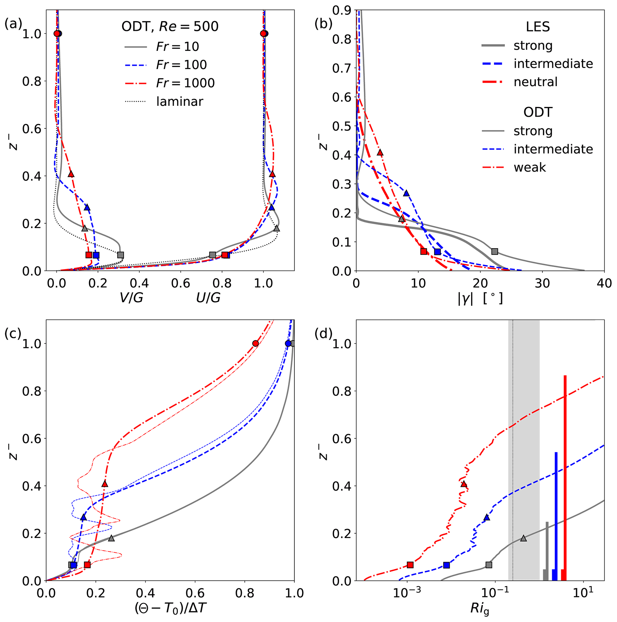
Figure 8 Synopsis of various simulated vertical property profiles. ODT results (solid and broken lines) at $t^{-}=\mathrm{4}$ have been obtained for W001 (N500 in panel b), I015, and S158 varying Fr for fixed Re=500. (a) Ensemble-averaged geostrophic U (right) and ageostophic V (left) velocity components together with the steady laminar Ekman flow solution (dotted) according to Eqs. (2) and (3). (b) Wind-turning angle of the ensemble-averaged velocity vector together with reference LES (thick lines) from Taylor and Sarkar (2008) for a slightly different case set-up and only approximately matching stratification regimes. (c) Ensemble-averaged (thick lines) and instantaneous (thin lines) temperature profiles. (d) Gradient Richardson number Ri_g of the ensemble-averaged state. The Ri_g=0.25 criterion (thin vertical line) and the widely accepted transitional margin $\mathrm{0.2}⩽{\mathit{Ri}}_{\mathrm{g}}⩽\mathrm{1}$ (shaded region) are given for orientation. Vertical bars (same color and order as profiles) mark the turbulence range of scales by the smallest and largest near-surface ODT eddy events that reach down into the viscous sublayer but do not touch the surface. Symbols mark the vertical locations z=D (□), δ_* (∘), and ${\mathit{\delta }}_{\mathrm{1}/\mathrm{2}}$ (△), respectively.

The velocity profiles shown in Fig. 8a suggest that the vertically propagating stratification is most influential on the high-level turbulence, which is consistent with the eddy JPDFs in Fig. 7. The mechanism is as follows. The near-surface stratification gradually diffuses into the mixed layer. At the surface, all near-surface eddies, from small to large scales, start to interact with the stratification and are influenced by it. The large-scale eddies are most influential on the turbulent mixing rate so that buoyancy damping has the largest sensible effect for the largest eddies. This is mimicked in ODT by complete rejection of large, almost marginal eddies that will no longer make it through the sampling procedure. This manifests itself by a laminarization of the flow, a reduction of the boundary layer thickness which is accompanied by a lowering, shrinking, and acceleration of the low-level jet which is consistent with the literature (e.g., Liu et al., 2021b; Maronga and Li, 2022). In ODT, the physical mechanism for low-level jet formation is as follows. For the ensemble-averaged state, flow laminarization due to the developing stable stratification is accompanied by a reduction of the boundary layer thickness. This leads to a lowering of the jet which is accompanied by an acceleration of the jet due to momentum and energy conservation. The acceleration is a transient phenomenon that appears as quasi-steady because the considered time interval is shorter than the Ekman time scale as noted above.

The inversion exhibited by the ensemble-averaged temperature profile and the “wiggly” nonmonotonic region of the instantaneous temperature profile are likewise reduced in height for stronger stratification. We attribute this to a reduction in mixing efficiency, which reduces together with the range of turbulence scales in the flow. In particular the stratification-induced suppression of large eddy events as shown by the eddy JPDFs in Fig. 7 significantly contributes to the reduction in turbulent boundary layer height.

In Fig. 8d, the gradient Richardson number Ri_g is shown in order to provide additional insight into the flow physics representation of the model. Theoretically, turbulence should only be maintained up to ${\mathit{Ri}}_{\mathrm{g}}⩽\mathrm{1}/\mathrm{4}$ as explained above, but due to local profile variability in a turbulent stratified shear flow, Ri_g can momentarily significantly differ from the idealized threshold that is based on the ensemble-averaged flow state. This is a correct representation of flow physics, similar to LES (Taylor and Sarkar, 2008, Figs. 13–15) and theory (e.g., Galperin et al., 2007; Zilitinkevich et al., 2013). For Ekman flow considered here, ${\mathit{Ri}}_{\mathrm{g}}\simeq \mathrm{1}/\mathrm{4}$ is reached for ${\mathit{\delta }}_{*}<\mathrm{1}$ so that turbulent fluctuations are not strictly constrained by $\mathrm{1}/\mathrm{4}$. This is suported by the near-surface turbulent eddies, which exceed the height $z_{\mathrm{1}/\mathrm{4}}^{-}\approx \mathrm{0.18}$, 0.38, 0.66 at which Ri_g=0.25 for Fr=10, 100, 1000, respectively. The range of boundary-layer turbulence scales is visualized by the smallest and largest near-surface ODT eddy events. (For each case, both of these eddies do not touch the surface but they are “anchored” in the viscous sublayer.) The same conclusion can be deduced from instantaneous temperature profiles shown in Fig. 8c by the fluctuation containing region, but this is far less definitive. So, in ODT as in various observations, the $\mathrm{1}/\mathrm{4}$ criterion gives an estimate for the height of the temperature inversion providing an approximation also to the upper bound for the size of the turbulence containing region of the stable Ekman boundary layer. Note that the thermal boundary layer length scale, ${\mathit{\delta }}_{\mathrm{1}/\mathrm{2}}$, falls below or at most marginally exceeds the $\mathrm{1}/\mathrm{4}$ criterion, hence, it provides another reasonable estimator for the stratification length scale of the stable boundary layer.

Last, Fig. 8b shows the wind-turning angle as defined in Eq. (25). ODT results are shown together with reference LES (Taylor and Sarkar, 2008) of a stable bottom Ekman layer. The case set-up differs in how the stratification is prescribed but the finite-time ODT and LES solutions are qualitatively comparable. By assuming outer layer similarity for the bulk, we compare ODT results to LES for approximately matching flow regimes. Therefore, in Fig. 8b, the red line shows the ODT solution for the case N500 rather than W001, but differences between the two cases are weak. It is remarkable how well the ODT and LES vertical profiles match given the differences in the model set-up, initial condition, and nominal Reynolds number. For neutral and strongly stable conditions, and under assumed outer layer similarity, the wind turning effects predicted by ODT are in reasonable agreement with the reference LES, whereas differences are notable for intermediate stratification. Towards the surface, differences in the wind-turning angle are expected because of the large difference in Re and the correspondingly large range of unresolved small scales within the LES for which the wall model plays a crucial role. In fact, LES from Taylor and Sarkar (2008) exhibit significantly lower wind-turning angles towards the surface than ODT. This discrepancy cannot be explained by finite Re effects and extrapolation of the surface drag law shown in Fig. 3b alone. This suggests that utilization of ODT as wall model has the potential to improve the representation of vertical and horizontal (geostrophic and ageostophic) transport processes in the vicinity of the surface.

5.4 Velocity hodograph and detailed statistics of the wind-turning angle

Figure 9 shows hodographs of the ensemble-averaged horizontal velocity components U(z,t) and V(z,t) together with corresponding reference DNS and the laminar Ekman spiral for orientation. The Ekman spiral is localized in the viscous log and sub-layer (which is in agreement with Ansorge and Mellado, 2014) so that near-surface flow properties and the boundary layer structure manifest themselves also in the hodograph. ODT does not fully reproduce the entire Ekman spiral, but it does capture wind-turning effects in the vicinity of the surface in terms of the Re dependence of the wall-shear angle γ_τ. The expected range of values of γ_τ follows from the parameterization shown in Fig. 3b. Here, we find that γ_τ≈20–30^∘ for neutral and weak stratification (Fr ≳ 1000), whereas ${\mathit{\gamma }}_{\mathit{\tau }}\to \mathrm{45}{}^{\circ }$ for very strong stratification (Fr<10, which is not investigated here) and complete near-surface laminarization. In between those values, the model exhibits a weaker tendency for laminarization than the reference DNS when Fr is decreased. One might speculate that this is related to less turbulent kinetic energy dissipation in the 1-D model than in 3-D DNS as shown in Fig. 4b, but the hodographs in Fig. 9 do not change much even if we sample after several inertial periods (not shown). In contrast to Navier–Stokes turbulence, ODT realizes a fully developed turbulent flow even at low Reynolds numbers due to its construction utilizing a simple mapping rule and “featureless” stochastic sampling of map applications. Therefore, the model exhibits resistance against leaving the developed turbulent state when stratification is applied as additional, energetic suppression mechanism. It is, therefore, understandable that the turbulent-laminar transition is not well captured by the model, even though it has the capability to completely cut-off turbulence on a physically justified, energetic basis.

Figure 9 Hodographs of the ensemble-averaged horizontal velocity $(U,V,\mathrm{0}{)}^{\mathrm{T}}$ at $t^{-}=\mathrm{1}$. ODT results (thin solid lines) are shown together with corresponding reference DNS (thick broken lines) from Ansorge and Mellado (2014). The wall-shear angle ${\mathit{\gamma }}_{\mathit{\tau }}\in [\mathrm{0},\mathrm{45}{}^{\circ }]$ represents the opening angle of the Ekman spiral. simulated values of γ_τ are explicitly given in the legend for comparison. The laminar Ekman spiral (curved dotted line) is characterized by ${\mathit{\gamma }}_{\mathit{\tau }}=\mathrm{45}{}^{\circ }$. Single points (symbols) have the same meaning as in Fig. 8.

Next, Fig. 10 shows detailed statistics of the wind turning angle γ at predefined heights. Reference observation data is based on the IGRA (Durre et al., 2006) and SPARC (Wang and Geller, 2003) radio sonde soundings in North America. Mid latitudes data from the ERA-Interim reanalysis (Dee et al., 2011) is used for comparison. Here we show the processed reference data according to Lindvall and Svensson (2019), who tested different definitions of the planetary boundary layer height, one with an interpolation to a predefined level, in order to extract the wind direction. This yields two curves for SPARC/IGRA and one for ERA-Interim. Level heights are taken at and above the planetary boundary layer thickness defined via the temperature inversion in the reference data, but at the Ekman layer thickness z=D in the present ODT simulations. This is justified for comparison based on the length scales and property profiles shown in Fig. 8. In order to obtain γ from ODT, Eq. (25) is evaluated for M high-resolution time series extracted at z=D, where the ensemble-averaged ageostophic flow velocity component V reaches its maximum. The probability density function (PDF) for γ is obtained from high-resolution time-series with $t^{-}⩾\mathrm{2}$ considering the entire M ensemble of flow realizations for the approximately statistically stationary state. ODT exhibits almost Gaussian but weakly skewed distributions of the wind-turning angle that shift to larger values but become narrower when Fr is decreased and Re increased. This is consistent with the results shown in Figs. 3 and 9.

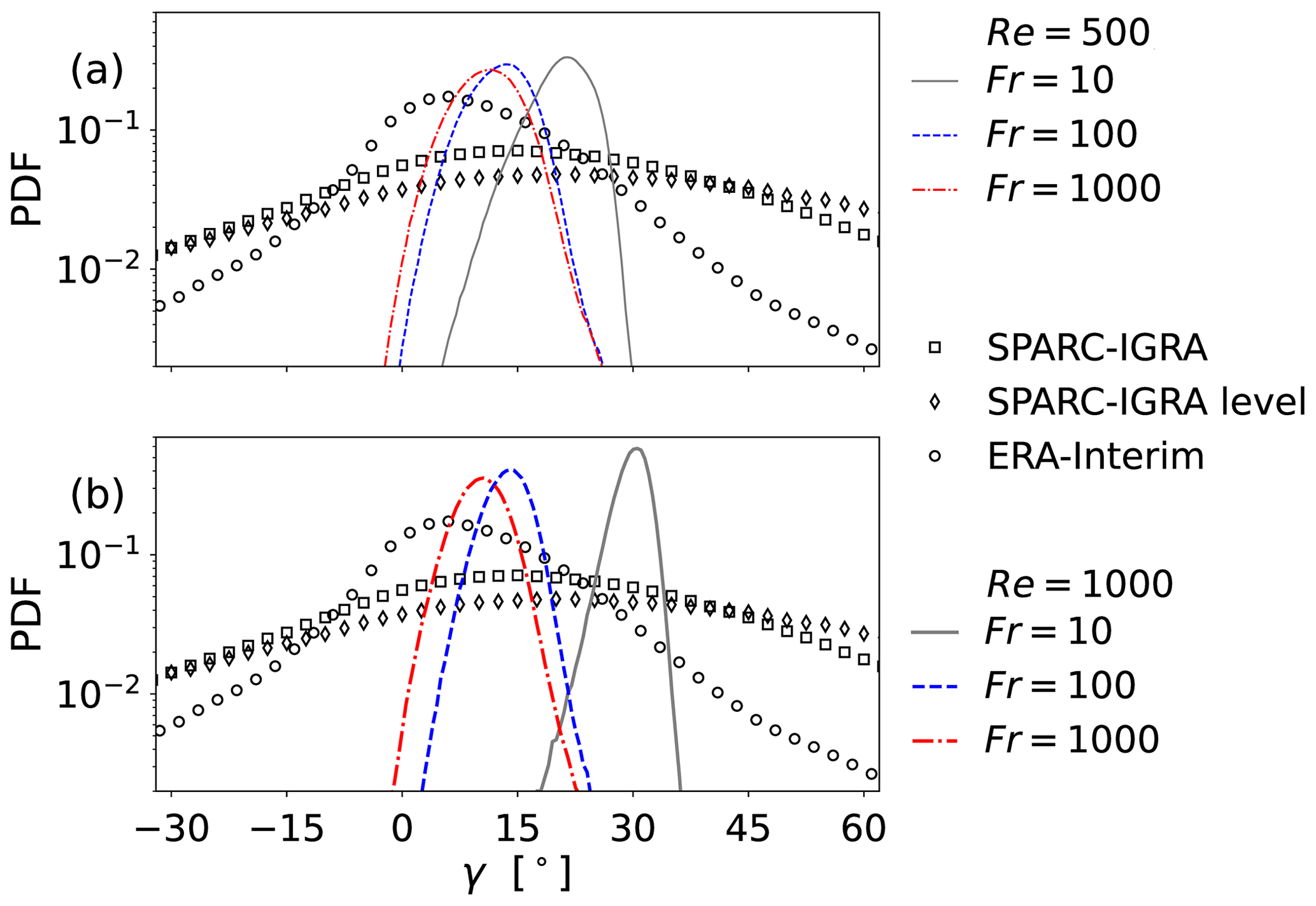
Figure 10 Probability density functions (PDFs) of the wind turning angle γ. In ODT, data was extracted at height z=D, which would be the thickness of the laminar Ekman layer. D is close to the location where the ensemble-averaged ageostophic velocity reaches its maximum. Reference data based on IGRA and SPARC soundings in North America and from an ERA-Interim reanalysis is shown for comparison. These reference data are taken from Lindvall and Svensson (2019), who performed the analysis by extracting horizontal velocity components at or at the level above the planetary boundary layer height.

The value range covered by the differently stratified ODT cases shown in Fig. 10 spans the central range where the mid latitudes observations and the reanalysis reach their maxima. Albeit the simple 1-D model captures only a small fraction of the angle distribution for any of the selected stratification cases, it is remarkable that the stratification ensemble formed by the three ODT cases approximately covers a broader range of angle variability than ERA-Interim does in the mid latitudes, which is a modeling bias (Lindvall and Svensson, 2019). Since stratification varies in the IGRA and SPARC observations, we suggest that ODT is able to capture a relevant fraction of the observed angle variability. Stand-alone ODT by itself, however, is unable to capture the tails of the angle distribution since it lacks information about the global and regional circulation patterns. Nevertheless, the accuracy of numerical models of the atmospheric boundary layer, including atmospheric chemistry applications, might be substantially improved by utilizing ODT as advanced wall model in each grid cell (Freire and Chamecki, 2021; Freire, 2022) since it is able to locally represent small-scale fluctuations and corresponding dynamical details of the flow.

5.5 Velocity boundary layer

In order to backup the above statement on the model's resistance against leaving the fully developed turbulent state, Fig. 11 shows boundary layer profiles of the normalized ensemble-averaged geostrophic velocity component $U^{+}\left(z^{+}\right)$. U⁺ and z⁺ are normalized with the momentary ensemble-averaged friction velocity u_* by evaluation of Eq. (12). We select $t^{-}=\mathrm{2}$ for the analysis in order to observe the short-time response to the stratification-induced buoyancy damping of turbulence after the system has settled. This is analogous to the LES of Taylor and Sarkar (2008) albeit no comparison with their data is done here. The linear and log layers are given by dotted lines using the same parameterizations as in Fig. 3a. The simulated boundary layer profiles shown in Fig. 11 exhibit inner layer similarity, which is indicated by the collapse on the linear viscous sublayer, Eq. (18), for $z^{+}<\mathrm{5}$. This is similar to Fig. 3a. For $z^{+}\gtrsim \mathrm{30}$, a log layer can be discerned but it is properly realized only for very weak stratification (Fr=1000) and $z^{+}\gtrsim \mathrm{100}$ for Re=1000. For stronger stratification (here Fr ⩽ 100), the log layer differs notably from the reference log law, Eq. (19). The lowering jet is a consequence of the stratification-induced elimination of large-scale near-surface eddies that govern the thickness of the turbulent boundary layer. The lower region of the log layer that is closer to the surface, however, is almost unaltered suggesting unaffected small-scale turbulence in the well-mixed near-surface region. This interpretation is supported the eddy JPDFs shown in Fig. 7.

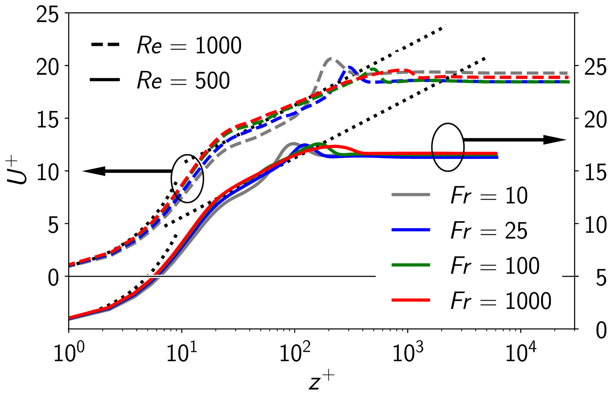
Figure 11 Velocity boundary layer after two inertial periods ($t^{-}=\mathrm{2}$) for various Fr and two Re showing the normalized ensemble-averaged geostrophic flow component U⁺. Baselines for cases with Re=500 (solid lines) and Re=1000 (broken lines) are offset by $\mathrm{\Delta }{U}^{+}=\mathrm{5}$ for better visibility. The empirical functions (dotted) are given for orientation and repeated from Fig. 4.

5.6 Buoyancy frequency

Finally, we assess the developing stratification itself as it affects also Ri_g discussed above. For this purpose, it is convenient to consider the buoyancy frequency N rather than the ensemble-averaged temperature Θ because N depends on the temperature gradient so it is indicative of force imbalances. Following Ansorge and Mellado (2014) for the case set-up described in Sect. 2, reference value T_r is taken at the surface z=0 as this will be reached for asymptotically large simulation times. For the ensemble-averaged temperature profile Θ(z) at fixed time t, the buoyancy frequency is given by

$$\begin{array}{}\text{(27)}& N=\sqrt{{\displaystyle \frac{g}{T_{\mathrm{0}}}}{\displaystyle \frac{\partial \mathrm{\Theta }}{\partial z}}},\end{array}$$

where temperature variations around the reference temperature, T_r=T₀, contribute only in the numerator. In the denominator we have $T_{\mathrm{0}}=\mathrm{\Theta }(\mathrm{0},t)$, which is the prescribed and fixed surface temperature after onset of the surface cooling.

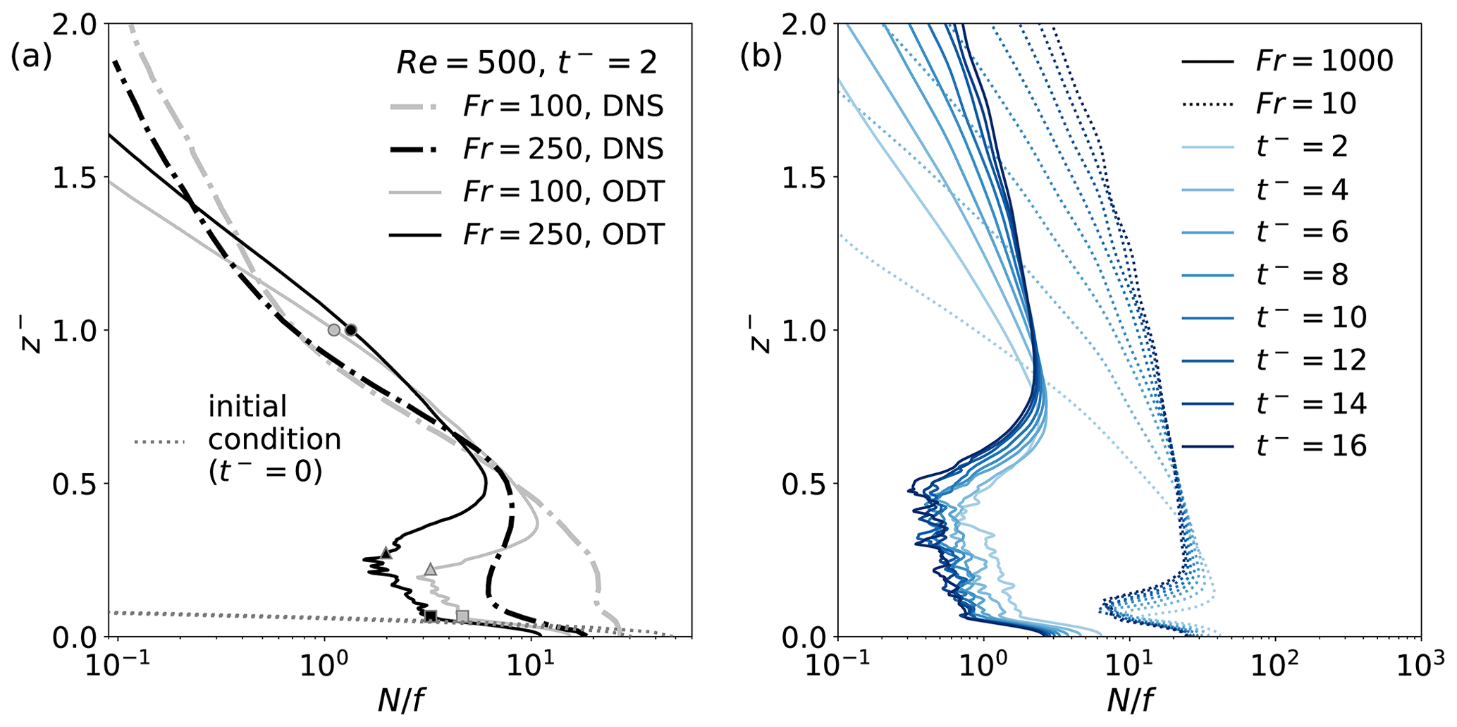
Figure 12 Vertical profiles of the normalized buoyancy frequency $N/f$. (a) Short-time simulation with comparison to reference DNS results at $t^{-}=\mathrm{2}$ for I015 and W006 with Re=500 at Fr=100 and 250, respectively. Corresponding reference DNS are from Ansorge and Mellado (2014) with a different Ri_B due to differences in the ODT and DNS velocity initial condition that manifest themselves by a difference in the turbulent boundary layer thickness ${\mathit{\delta }}_{*,\mathrm{0}}$ (see Table 3). (b) ODT prediction of the long-time evolution of the buoyancy frequency for weak and strong stratification cases W001 and S158 shown in Figs. 5 and 6, respectively. “Wiggles” are due to finite sample variability. Note that the horizontal axis is scaled differently in panels (a) and (b).

Figure 12 shows simulated vertical profiles of the normalized buoyancy frequency $N/f$ for short and long simulation times. Long-time simulations reach a statistically stationary transient due to slow molecular diffusion of the temperature perturbation into the bulk. For the latter, no reference DNS are available due to cost constraints that are overcome with ODT. For short-time simulations, ODT results are shown together with corresponding available reference DNS from Ansorge and Mellado (2014) for the weak (W006) and intermediate (I015) stratification at low Re=500. The buoyancy frequency is evaluated after two inertial periods ($t^{-}=\mathrm{2}$) from the onset of the surface cooling, which is after the initial transient has passed based on the ensemble-averaged temperature profiles Θ(z). The initial condition is due to the prescribed temperature profile given in Eq. (1), which is identical for ODT and DNS and given for orientation. The stratification has evolved from the initial to the current state and keeps on evolving in the outer region $z^{-}\gtrsim \mathrm{1}$. The ODT near-surface “wiggles” also change in time due to finite sample variability of the selected M ensemble. While ODT broadly captures the vertical structure of the buoyancy frequency, the model notably underestimates $N/f$ in the well-mixed layer in the vicinity of the surface. The well-mixed layer lies in between $z^{-}\approx \mathrm{0.05}$ and $z^{-}\approx \mathrm{0.25}$ (0.30) for Fr=100 (250). This means that the triplet-map-based turbulent advection modeling, at least for low Re, yields stronger turbulent stirring than the DNS. This results in a more homogeneous near-surface mixed layer in ODT as indicated by a more uniform vertical profile Θ(z) and, hence, smaller values of $N/f$. Since the velocity shear is comparable in ODT and DNS, lower $N/f$ in ODT implies lower Ri_g. This is consistent with the assertion that fully developed (“featureless”) turbulence is the preferred state of the ODT solution as discussed above.

Note, however, that the buoyancy frequency recovers for $z^{-}\approx \mathrm{0.5}$ so that ODT and DNS exhibit better agreement towards the top of the boundary layer ($z^{-}\simeq \mathrm{1}$) where turbulence is absent. Well above the boundary layer, for $z^{-}\gtrsim \mathrm{1.5}$, the buoyancy frequency in ODT is again underestimated but this cannot be due to turbulent mixing as there is no turbulence and, correspondingly, are no ODT eddy events in this region. Apart from not fully captured turbulent mixing across the boundary layer, it is likely that differences in the case set-up, that is, differences in the initial condition, explain this feature. We remind of the mismatching values of Ri_B (see Table 3), which seems to support the latter hypothesis since the turbulent boundary layer thickness ${\mathit{\delta }}_{*,\mathrm{0}}$ is in fact larger in ODT than in the reference DNS. Other unresolved flow features, like inertia-gravity waves (Maronga and Li, 2022) or spatial intermittency patterns (Ansorge and Mellado, 2016), might also contribute to the observed discrepancy.

6 Conclusions

Turbulent Ekman flow over a smooth surface and its reaction to developing stratification due to a sudden surface cooling is investigated as canonical problem for polar and nocturnal boundary layers over land or ice. Here, the stochastic one-dimensional turbulence (ODT) model has been used as numerical tool in order to explore stratification effects and their effects on turbulence scales, including flow statistics. Various observables have been considered encompassing instantaneous and ensemble-averaged velocity and temperature profiles, bulk quantities, derived and surrogate variables. The emphasis is on the wind turning effect and its variability which are both numerically challenging, requiring high-fidelity models. Wind-turning effects are intimately related to cross-isobaric mass transport, which has been reported to be underestimated in numerical circulation models as demonstrated recently by reanalysis data of the mid latitudes (Lindvall and Svensson, 2019).

In the present study, the ODT model aims to resolve all relevant scales of the turbulent flow but only along a vertical coordinate for a columnar computational domain. Molecular diffusion and Coriolis forces are directly resolved, whereas the effects of turbulent stirring motions are modeled by a stochastic sequence of discrete eddy events that punctuate the deterministic diffusive flow evolution. Two adjustable model parameters were calibrated for neutral conditions utilizing reference data for the surface drag law. Either the friction velocity or the surface wind-turning angle can be matched by two different sets of model parameters. Model parameter adjustment is advisable when the flow regime changes from low Re ≲ 1000 to high Re ≳ 1000 since the laminar Ekman layer length scale (thickness) moves from below to within the asymptotic logarithmic region of the turbulent boundary layer. This suggests that model parameters close to C≃6 and Z≃1 are applicable to high asymptotic Reynolds numbers, which will enable forthcoming analyses of transient high-Re atmospheric boundary layers (e.g. Meneveau and Marusic, 2013; Huang et al., 2021) and some associated turbulent flow features (like locally uniform momentum zones and microfronts, de Silva et al., 2016; Sullivan et al., 2016) in stable atmospheric boundary layers by utilizing ODT as a regime-spanning but cost-efficient flow model.

The model application to the stratified cases was performed with fixed model parameters. Present results demonstrate that ODT is able to very reasonably capture the structure of the viscous and thermal boundary layer for weak and strong, but not for intermediate stratification. We assert that this is by construction and the model is unable to accurately capture the laminar-turbulent transition except when changing from a fully laminar to a fully turbulent flow regime. An analysis of the turbulence spatial scales based on model surrogate data and conventional flow statistics revealed that ODT prefers fully-developed turbulence already at low Reynolds numbers. The stratification is initially localized at the surface and propagates upwards interacting with neutral Ekman flow turbulence. The model suggests that the flow reacts by energetically cutting-off first the large-scale near-surface eddies responsible for outer layer turbulence due to which the inversion and near-surface jet lowers for stronger stratification. By contrast, small-scale near-surface eddies in the well-mixed turbulent surface layer remain almost unaffected. This is consistent with flow physics (e.g., Ansorge and Mellado, 2014) with the sole exception of the representation of transitional (low Reynolds number) turbulence.

Furthermore, we have shown that, albeit ODT is able to qualitatively capture surface wind-turning effects for various stratified conditions (Fr) and wind speeds (Re), the model underestimates the ageostrophic flow component and, hence, Ekman transport. The simulated Ekman spiral mimics that of a more turbulent case. This supports the assertion that the model, due to its construction, yields fully developed turbulence properties already for weak turbulence intensities so that it can only qualitatively capture the laminar-turbulent transition for the stable boundary layer flow. This limitation is presumably less of a problem when ODT is utilized as advanced subgrid-scale model (Gonzalez-Juez et al., 2011b; Glawe et al., 2018) or wall model (Schmidt et al., 2003; Freire, 2022) within an LES approach. It is remarkable that three ODT cases for weak, intermediate, and strong stratification, cover a broader range of wind-turning angle variability than a reanalysis for the mid-latitudes. The reanalysis in fact misses small-scale variability. This is, of course, not a fair comparison since stand-alone ODT does not capture the broad range of observed wind turning angles. Nevertheless, it is a motivation to give ODT further consideration to more accurately represent the variability and flow physics of subgrid-scale turbulent processes in atmospheric circulation models. This more accurate subgrid-scale representation is attained by a vertical-column formulation that is highly resolved in space and time, offering future opportunities for improved treatment of multi-physics processes such as mixing-dependent atmospheric chemistry in stand-alone as well as subgrid ODT formulations.