 | 02 Jan 2024
Probabilistic end-to-end irradiance forecasting through pre-trained deep learning models using all-sky-images
Sebastian Houben
Stefanie Meilinger
This work proposes a novel approach for probabilistic end-to-end all-sky imager-based nowcasting with horizons of up to 30 min using an ImageNet pre-trained deep neural network. The method involves a two-stage approach. First, a backbone model is trained to estimate the irradiance from all-sky imager (ASI) images. The model is then extended and retrained on image and parameter sequences for forecasting. An open access data set is used for training and evaluation. We investigated the impact of simultaneously considering global horizontal (GHI), direct normal (DNI), and diffuse horizontal irradiance (DHI) on training time and forecast performance as well as the effect of adding parameters describing the irradiance variability proposed in the literature. The backbone model estimates current GHI with an RMSE and MAE of 58.06 and 29.33 W m−2, respectively. When extended for forecasting, the model achieves an overall positive skill score reaching 18.6 % compared to a smart persistence forecast. Minor modifications to the deterministic backbone and forecasting models enables the architecture to output an asymmetrical probability distribution and reduces training time while leading to similar errors for the backbone models. Investigating the impact of variability parameters shows that they reduce training time but have no significant impact on the GHI forecasting performance for both deterministic and probabilistic forecasting while simultaneously forecasting GHI, DNI, and DHI reduces the forecast performance.
- Article
(16184 KB) - Full-text XML
-
Supplement
(28356 KB) - BibTeX
- EndNote


Model predictive control (MPC) of renewable energy systems relies on accurate predictions to correctly optimize the trajectory of the systems control actions (Riou et al., 2021; Maheri, 2014; Sachs and Sawodny, 2016; Dongol, 2019; Zhu et al., 2015; Tazvinga et al., 2013; Taha and Mohamed, 2016; Zhang et al., 2018; Mbungu et al., 2017). While some system components can be modeled using physics-based approaches, forecasting the electrical load and meteorological parameters in real-time remains a challenge. Several approaches can be used to generate these forecasts. Among them are statistical, empirical, numerical, and artificial neural network (ANN) methods (Sachs, 2016; Dongol, 2019; Bozkurt et al., 2017; Bouktif et al., 2018; Yang et al., 2016; Maitanova et al., 2020; Telle et al., 2020; Bruno et al., 2019; Chaaraoui et al., 2021). ANNs have gained popularity in a variety of applications such as image classification, action recognition, and time-series forecasting. They have shown improved performance and robustness, compared to statistical and physics-based approaches (Krizhevsky et al., 2012; He et al., 2015; Tan and Le, 2020; Devlin et al., 2019; Shoeybi et al., 2020; Brown et al., 2020; Radford et al., 2019; Qian et al., 2021). This trend led to the development of ANNs that use images from all-sky imagers (ASI) to predict the future solar irradiance. Current solutions consist of stand-alone ANN applications or a combination of ANN and physics-based approaches (Pothineni et al., 2019; Paletta et al., 2021; Yang et al., 2021; Fabel et al., 2022; Nouri et al., 2021; Hasenbalg et al., 2020). In addition, training ANNs with parametric or non-parametric uncertainties can provide information through symmetric probability distributions. Xiang et al. (2021) use a quantile regression method to determine the probability distribution, by defining a set of 19 evenly distributed quantiles as output of their ANN. Paletta et al. (2022), treats their ANN forecasting model as a classifier to generate binned probability classes, by defining 100 output classes which are equally distributed throughout their irradiance normalization range. Feng et al. (2022) use Bayesian model averaging (BMA), which requires a set of ANN models. They differ in the input images they receive, which are augmented through occlusion perturbations, resulting to a global horizontal irradiance (GHI) forecast ensemble. This ensemble is then used to estimate parameters of a probability density function (PDF), defining a normal distribution. Nie et al. (2023) propose a new hybrid approach, by combining a stochastic generative pre-trained transformer ANN and a physics-informed ANN for video prediction. An ensemble of possible image sequence predictions for each time step is generated, based on past images from an ASI. The predicted sequence ensembles are then used to estimate a GHI probability distribution through another ANN for each future time-step. Nouri et al. (2023) propose a more conservative approach, using a U-Net ANN for cloud segmentation and a stereoscopic cloud height estimation with two ASI. With a sequence of ASI images, the authors can then determine the cloud movements and extrapolate the expected direct normal irradiance (DNI) through ray-tracing and a sun tracker measurement device, which decomposes the observed solar irradiance in its diffuse and direct components. The authors combine their method with a persistence forecasting method to enhance the forecast. To obtain probabilistic forecasts, the authors classify the past 15 min of irradiance data into eight variability classes. The variability classes are formalized through a set of variability parameters defining value boundaries for each variability class. Depending on the forecast horizon, the authors use past observations and/or deterministic forecasts for the variability classification in a sliding window fashion. To determine which variability class represents which probability distribution, the authors use approximately 2 years of observation data and simulate forecasts on this data. By logging the forecast error and the corresponding variability class, the authors then determine a discretized probability distribution for each variability class, based on the magnitude of the forecast error. These discretized probability distributions are then stored in a look-up table and fetched as reference when performing forecasts on the validation data set, by determining the variability class with the above mentioned method.
Probability information can be harnessed in probabilistic Model Predictive Control (MPC) applications for renewable energy systems, enabling the incorporation of uncertainty into the state estimation, as well as the constraining and fine-tuning of control parameters (Sachs, 2016). Deploying current methods to perform such probabilistic forecasts through ASI increases both investment and maintenance costs, attributed to the need for irradiance measurement instruments like sun trackers or pyranometers (Nouri et al., 2021, 2023; Paletta et al., 2021). Furthermore, the prediction of a large number of parameters to define the probability distribution, or the training and inference of multiple models to estimate a smaller number of parameters, both either impact the models performance by distributing ANN model parameters on a large set of output neurons or proportionally increases training and inference time depending on the size of the ensemble required. The exploitation of transformer models to predict image sequences can be a viable approach, but appears to use more computational resources than required by using the predicted images as a bridge to lower resolution outputs. Also, using asymmetric probability distributions appears to be more suitable for our use case, rather than symmetric ones (Barnes et al., 2021; Feng et al., 2022).
In this research, we propose a method to exploit an ImageNet pre-trained ResNet50v2 backbone as a feature extractor for probabilistic ASI-based irradiance forecasting of up to 30 min. The feature extractor allows us to output irradiance values with minor modifications. The method consists of two stages. First, the backbone is trained to predict four parameters from an ASI image, defining an asymmetric irradiance probability distribution. Afterwards, we extend and retrain the model to perform the forecasting task using long short-term memory (LSTM) and densely connected layers. Therefore, our method uses a two-stage training process, but performs inference with a one-stage model. Our method also facilitates the easy substitution of the feature extractor backbone with more powerful or more efficient models, such as MobileNet, DarkNet, EfficientNet or ConvNeXt (Howard et al., 2017; Redmon and Farhadi, 2018; Tan and Le, 2020; Liu et al., 2022). We add relevant exogenous variables from literature (Paletta et al., 2021; Yang et al., 2021) and investigate the impact of variability parameters, proposed by Schroedter-Homscheidt et al. (2018), instead of constraining the problem within variability classes, as done by Nouri et al. (2023), allowing the ANN to determine suitable parameters for performing the forecast. The impact of adding DNI and diffuse horizontal irradiance (DHI) on the forecasting and estimation performance is investigated.
Unlike previous work, we avoid predicting complex high-dimensional outputs to determine distributions, or compute-intensive ensembling techniques and instead restrict our output to four parameters which are sufficient to fully define the asymmetric probability distribution as a continuous function and train only one model in two stages, instead of an ensemble of models. Our approach only needs a single ASI and requires a radiometer only for training. It can be deployed without the usage of a radiometer, greatly reducing maintenance and investment costs for the implementation on the field. We report training and inference times, to determine the models potential for edge computing applications for MPC, and estimate the effort to train our model on a much larger and geographically diversified data set. The following research questions are addressed in this study:
-
Can pre-trained ANNs be adapted to estimate the GHI from an ASI image?
-
How much training time is required?
-
Does adding the DNI and DHI to the estimation task improve the accuracy of GHI estimates?
-
Is it possible to generate irradiance probability distributions instead of deterministic values?
-
Can the estimation task be extended to a forecasting task?
-
What is the impact of adding the variability parameters proposed by Schroedter-Homscheidt et al. (2018)?
-
Are the forecasts and estimations generated within acceptable inference times?
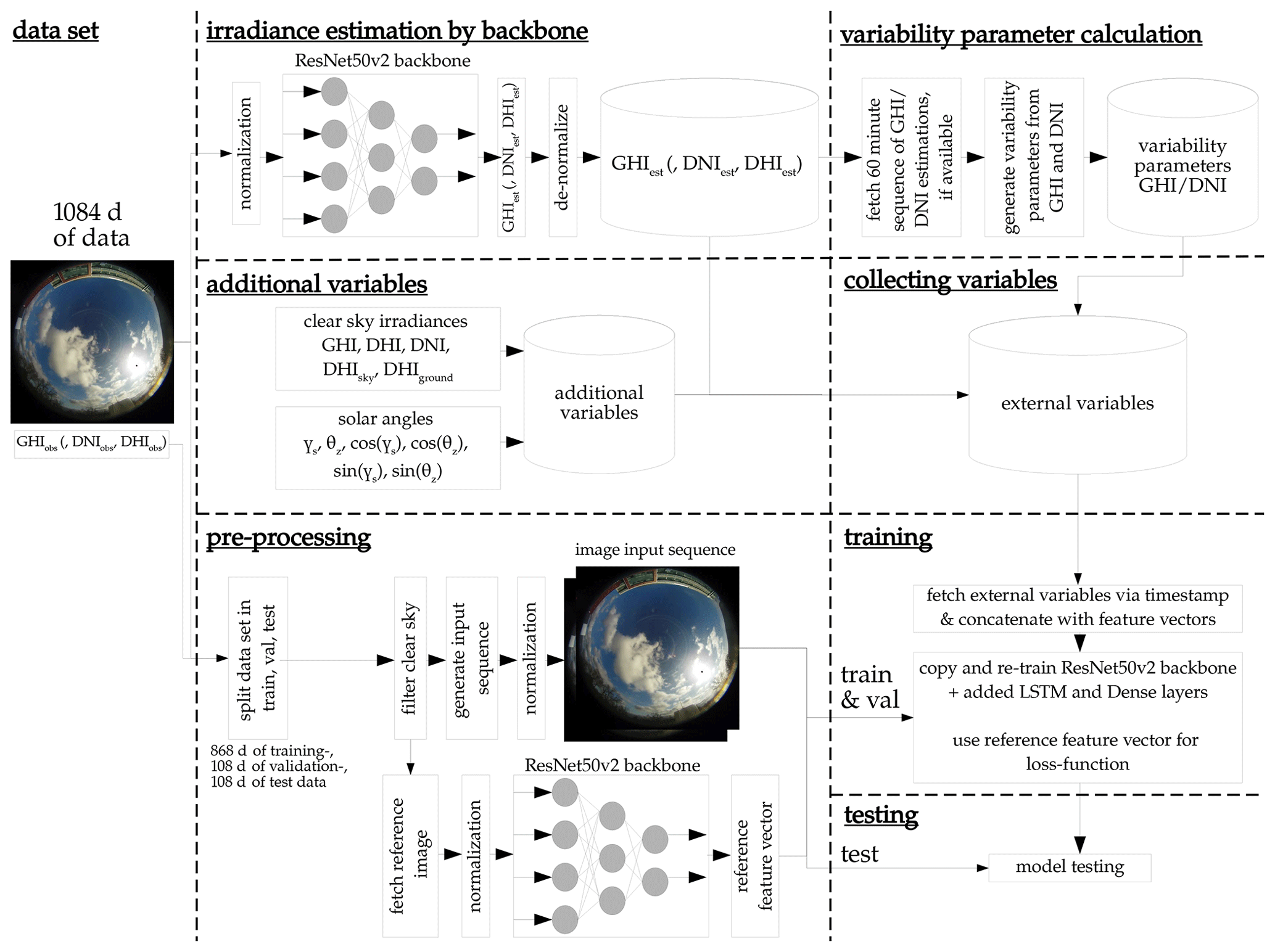
This research uses an open data set provided by Pedro et al. (2019). The data set contains a quality-controlled record of the GHI, DNI, DHI measurements and corresponding ASI images. The data ranges from 2014 to 2016 with a temporal resolution of 1 min and has been collected in Folsom, California. For our application, the image resolution is scaled down to 224×224. To avoid trivial cases with no cloud coverage, the majority of clear-sky data points were filtered out with the clear-sky identification method proposed by Reno and Hansen (2016). Additionally, data points were flagged as clear-sky 30 min prior and after detection to ensure that the model did not predict clear-sky data points, focusing in this study on the prediction of the more challenging non-clear-sky events. For the forecasting task, we also ensured that ASI images for the past hour were available to calculate the variability parameters, proposed by Schroedter-Homscheidt et al. (2018). From the set of ASI images, we then generated irradiance values from the backbone models. This research follows the assumption that there is no radiometer available during the operation of the system. We therefore exploit the ASI as a radiometer. The data set was randomly separated into 868 training days, 108 validation days, and 108 testing days. Timestamps of the ASI images were rounded to the full minute since the images were not taken exactly to the same minute as the irradiance measurements.
In this section, we present the two-stage training approach, first introducing the backbone model in Sect. 3.1. The variability parameters, proposed by Schroedter-Homscheidt et al. (2018), are presented in Sect. 3.2. The extension of the backbone to a forecasting model is described in Sect. 3.3. Architectures and training configurations are documented for both stages. For comparison purposes, we use four backbone model variations. The first variation only estimates the deterministic GHI. The second estimates GHI, DNI, and DHI simultaneously. The last two variations output asymmetric probability distributions instead of deterministic values.
The forecasting model has an additional variation, adding the aforementioned variability parameters. This variation serves to determine their impact on performance. The variability parameters are calculated through the backbone model's past and current irradiance estimations from the ASI images. Forecasting horizons of 5, 10, 20, and 30 min were evaluated for each forecasting models variation, considering horizons investigated in literature and seamless prediction applications with numerical weather prediction methods (Pothineni et al., 2019; Nouri et al., 2021; Xiang et al., 2021; Paletta et al., 2021; Feng et al., 2022; Diagne et al., 2012; Kober et al., 2012; Owens and Hewson, 2018; Urbich et al., 2020).
3.1 Backbone model
The ResNet50v2 ANN architecture proposed by He et al. (2016) is used as a classifier. It distinguishes a set of classes describing the content of an image. The model is trained on the ImageNet data set to validate its performance compared to other architectures (Deng et al., 2009). Minor modifications to the architecture allow the model to be exploited as a feature extractor. This approach is practiced in other disciplines (Rezende et al., 2017; Ou et al., 2019; Ronneberger et al., 2015). Furthermore, a pre-trained model already learned to extract features within images to perform its task. Features can include edges, corners, or color gradients. The model can therefore be deployed to perform other tasks requiring a similar set of features (Ferreira et al., 2018; Du et al., 2018).
In the first step, we modified a pre-trained ResNet50v2 model by removing the output layer after the 5th convolutional block. This step reveals the feature vector, where each element describes a lower level representation of a certain image section. These representations help the ANN fulfill its task. They are not pre-defined and the ANN determines which feature it requires to generate the desired output from the image. A pre-trained ResNet50v2 model had already learned to extract a set of these low level representations from a classification task, a process that was helpful for the investigated application. A two-dimensional global average pooling layer serves to reshape the feature vector to appropriate dimensions (Chaaraoui et al., 2022).
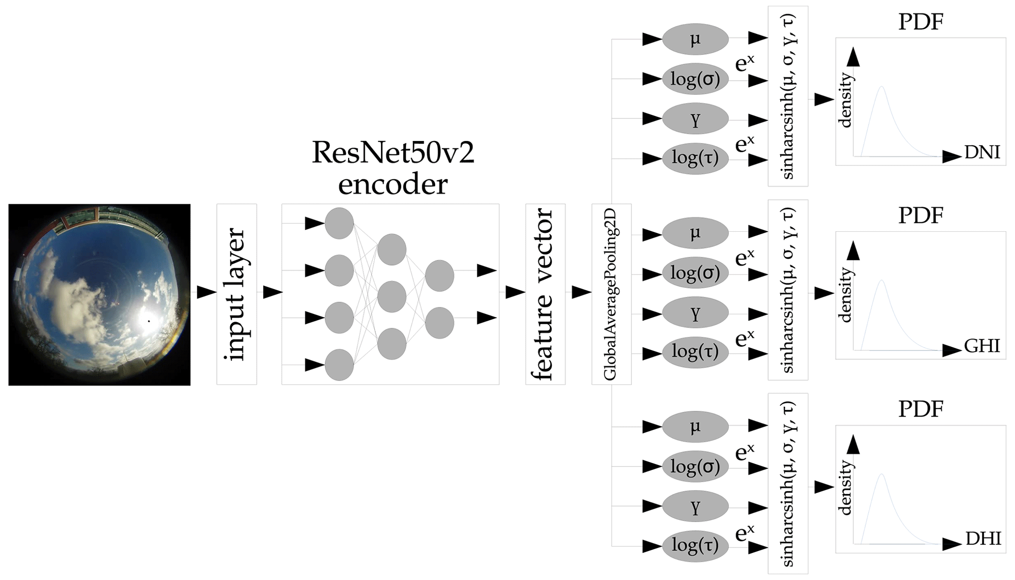
Figure 1Architecture of the backbone ANN, which generates asymmetric probability distributions for all three irradiance components.
To transfer the classification task to a probabilistic regression, we use an approach proposed by Barnes et al. (2021). The output layer is replaced by four densely connected neurons representing the four parameters location (μ), tailweight (τ), skewness (γ), and scale (σ). These parameters define a sinh-arcsinh distribution, proposed by Jones and Pewsey (2009), which allows for asymmetric probability distributions to be flexibly defined. μ defines the location of the irradiance distribution and gives an estimate of the solar position and its coverage by a cloud. σ scales the distribution and plays a major role in representing the models confidence. τ and γ allow the model to create asymmetries, by altering the distribution's skewness and kurtosis. We expect this asymmetry to be especially helpful with this particular forecasting task, simply by taking into account that certain cloud cover situations have a higher probability to decrease (current irradiance is close to clear-sky) or increase (current irradiance is the result of a cloud blocking the sun) the solar irradiance.
To maintain unsigned values for τ and σ, their logarithm is calculated with log (τ) and log (σ) as a bijective map. This bijective map constrains the ANN to output only positive values for these two parameters, because a negative tailweight or negative spread of the distribution are not possible. The exponential function of the corresponding outputs returns τ and σ. The backbone architecture is illustrated in Fig. 1.
The task of the probabilistic backbone model is to estimate the probability distribution of the GHI, DNI, and DHI from an ASI image. For that, we first train the model to understand the relation between the image and the irradiance values, before moving over to a forecasting task.
To examine the performance differences between this probabilistic approach and a deterministic approach, we exchange the layers after the global average pooling layer for a set of densely connected neurons. These neurons output a deterministic irradiance value. This deterministic architecture is shown in Fig. 2.
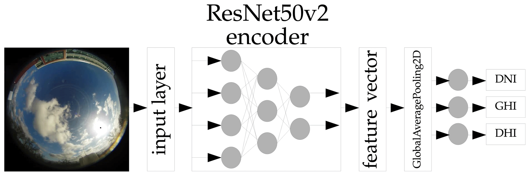
Figure 2Principle of the backbone ANN architecture to generate the deterministic irradiances for all three irradiance components.
To output only the GHI, the top and bottom output branches after the global average pooling layer for DNI and DHI are removed.
3.1.1 Backbone model training configuration
A mirroring strategy is applied for our multi GPU system, replicating the models on each GPU and dividing the batch among them. The weight update is performed after each training step, by aggregating the gradients of all four replicas. Data shuffling is applied for each epoch as an augmentation technique. As a loss function, we implement the negative logarithmic likelihood for the probabilistic models, as suggested by Barnes et al. (2021) and defined as:
with xi being the ith input from the batch input of the ANN, yi being the corresponding real irradiance value and 𝒫 the probability density function of the sinh-arcsinh function, which is defined by the parameters μ, σ, γ, and τ. The deterministic models compute the loss with the mean squared error (MSE), defined as:
with being the output of the ANN. Note that the losses of the models predicting GHI, DNI and DHI simultaneously are equally weighted among the irradiance components.
The weights are optimized with the adaptive moment estimation optimizer (ADAM). While the deterministic models use a learning rate reducer and early stopper, the probabilistic configurations do not use the early stopper, due to the low number of epochs necessary to train the models.
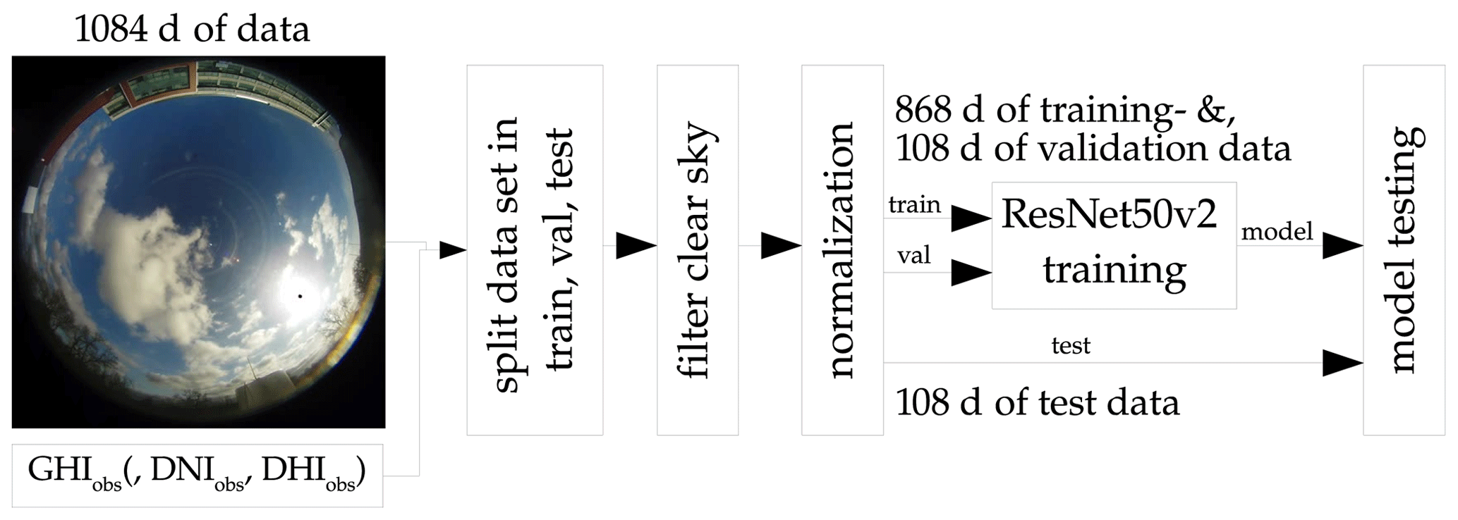
Table 1Training configurations for the backbone models.
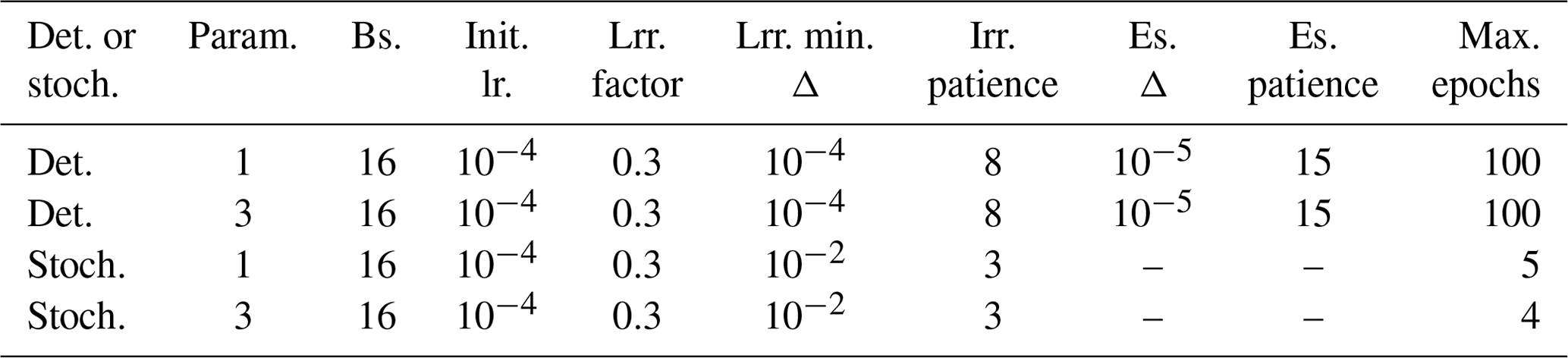
Det.: deterministic; stoch.: stochastic; Param.: either GHI-only or GHI, DNI and DHI simultaneously; Bs.: batch size; Init. lr.: initial learning rate; Lrr.: learning rate reducer; Es.: early stopper.
Figure 3 shows the training pipeline of the backbone ANN model. The image is preprocessed by scaling the pixels to values between −1 and 1 (Abadi et al., 2015). The irradiance values are normalized, with:
Parameters for all four configurations can be found in Table 1.
3.2 Variability Parameters
Schroedter-Homscheidt et al. (2018) utilize variability parameters from relevant literature to classify 1 h of minutely radiation time-series in eight variability classes. These variability classes serve as indicators for different cloud situations, which differ in their impact on solar power production. In our study, we use these variability parameters as additional features for our forecasting model to determine, if they have an impact on forecasting performance. All variability parameters are derived from the GHI and DNI, unless stated otherwise, resulting into 15 variability parameters from the GHI and 13 variability parameters from the DNI:
-
σSk, proposed by Skartveit et al. (1998), uses the clear-sky index of the current, past and future observation and computes root mean squared differences. Schroedter-Homscheidt et al. (2018) use a sliding window approach to first determine the hourly mean clear-sky indices throughout the time-series and then apply the equation by Skartveit et al. (1998), defined as:
-
VCoimbra, proposed by Coimbra et al. (2013), resembles the root mean squared difference between the clear-sky index and the clear-sky index one time step ahead, with:
-
VIStein, proposed by Stein et al. (2012), divides the sum of the root squared difference between the current and previous irradiance with the root squared difference between the current and previous clear-sky irradiance:
-
Using the variability indices proposed by Perez et al. (2011), which takes the absolute differences between two consecutive clear-sky indices and irradiance values throughout the whole hour and calculates the mean, standard deviation and maximum value within the sequence of differences, defined as:
-
OVER5 and OVER10, representing the occurrences of GHI overshoots within the time-series sequence, only counting either 5 % or 10 % over clear-sky as overshoot occurrence:
This variability parameter is only applied for GHI values, since overshoots are theoretically not possible with DNI.
-
Counting the changes in the sign of the first derivative (CSFD) in the time-series sequence, proposed by Kraas et al. (2013), where only those changes are counted which show a 15 % change between one local extreme to the other.
-
Using a time-series envelope function, proposed by Jung (2015). Initially the irradiance time-series is divided into overlapping sub-sets of the time-series, each spanning a duration of 4 min. We then identify the minimum and maximum of each sub-set. These points initially form the preliminary upper and lower envelopes, respectively. These sub-sets are then extended by 1 min from the original time-series sequence until a new minimum or maximum is identified, substituting the previously defined minimum or maximum of each sub-set. By methodically applying this process to each 4 min subset across the entire time series, we establish two new time-series – the upper and lower envelopes. These envelope series effectively encapsulate the original irradiance time-series. Using these two envelope time-series, Schroedter-Homscheidt et al. (2018) calculate three variability parameters:
-
The mean of each delta of the upper and lower envelope time-series UML (Upper Minus Lower).
-
The mean of each delta between the upper envelope time-series and corresponding clear-sky radiation UMC (Upper Minus Clear).
-
The mean of the lower envelope time-series LMA (Lower Minus Abscissa).
-
With the variables in the above mentioned equations as:
-
the number of elements in the time-series sequence N.
-
g is the radiation component used to calculate the variability parameters. Which component is used, depends on the architecture used in Sect. 3.3.
-
gcs is the clear-sky value, calculated with the clear-sky model by Perez et al. (2002).
-
kc is the clear-sky index of the corresponding radiation component “rad” used in the equation.
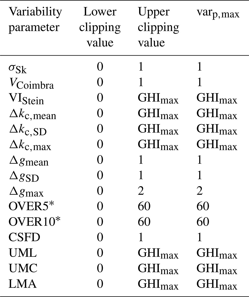
The variability parameters are clipped and normalized according to the values shown in Table 2. The values are normalized, with:
Table 2Clipping and normalization values for variability parameters. * – only for variability parameters derived from GHI.
3.3 Forecast model
We extend the backbone model to perform a forecasting task, by outputting the feature vector for the current time step t and the past time step t−n from the backbone, with n being the forecasting horizon. These feature vectors are then concatenated to predict the future feature vector at time step t+n, using a set of LSTM and densely connected neuron layers. To translate the predicted feature vector to a deterministic or probabilistic irradiance, we use the approach from the backbone model, shown in Fig. 1 (probabilistic) and Fig. 2 (deterministic).
Figure 4 illustrates the probabilistic approach we address in this section. This configuration outputs the GHI, DNI, and DHI simultaneously. The architectures for the probabilistic GHI-only model and the corresponding deterministic models can be found in Appendix A. These architectures follow an analogous concept to the approach explained here. The backbone model is trained beforehand, as described in Sect. 3.1. The model is divided into four components (a), (b), (c), and ().
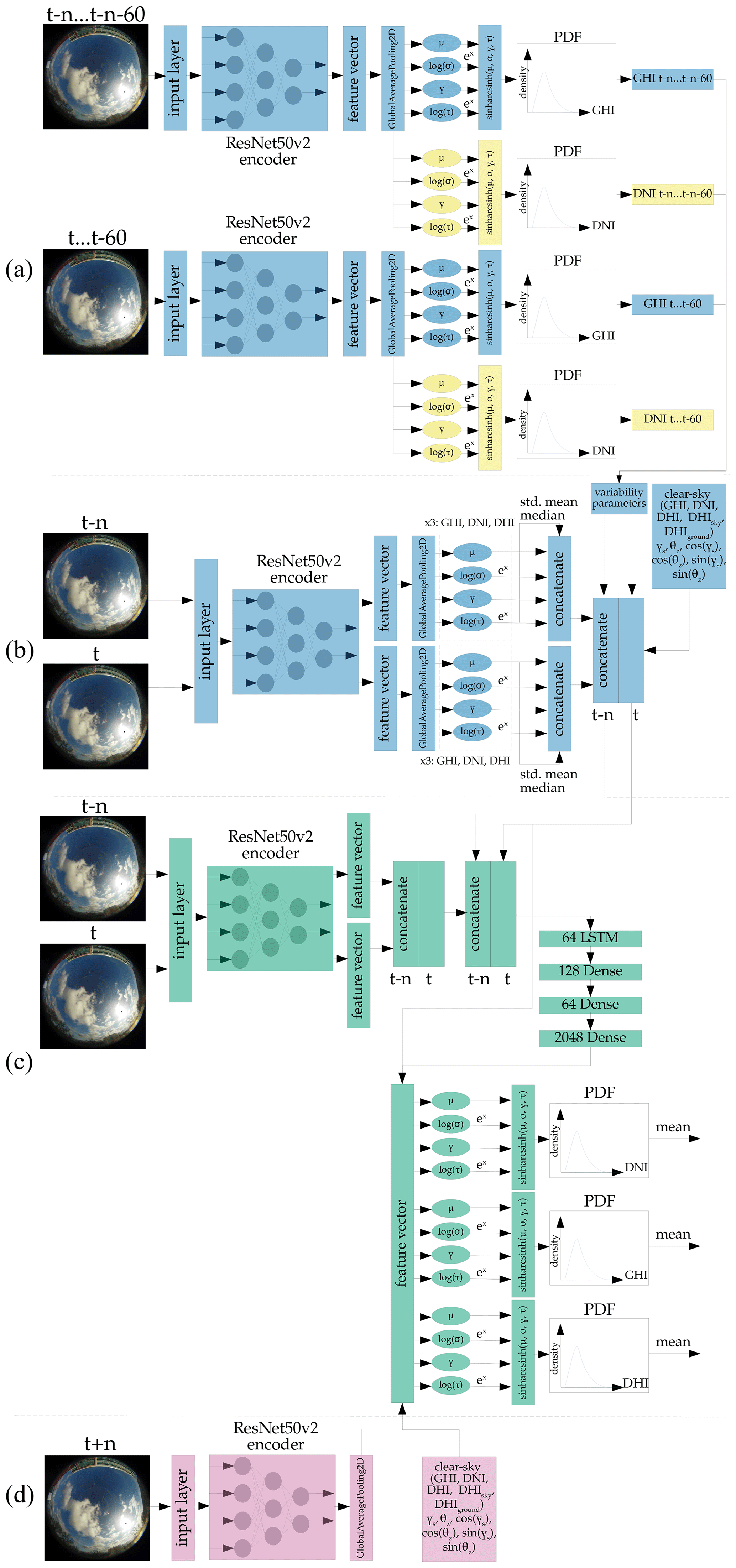
Figure 4Architecture of the probabilistic forecast model, forecasting the probability distribution of the GHI, DNI, and DHI. Blue - not trained, but part of training; green – trained; pink – not trained and not part of training; yellow – not trained, part of training, and optional.
Figure 4a shows how the variability parameters proposed by Schroedter-Homscheidt et al. (2018) are generated. These parameters are added later to our feature vectors. The variability parameters are derived from a sequence of GHI and DNI values from ASI images of the past time steps t to t−60 min and t−n to min, with n being the forecasting horizon. The deterministic GHI and DNI are estimated by the previously described probabilistic backbone model shown in Fig. 1. To obtain explicit values from the probabilistic distributions, the expectation μmean of the distribution is analytically calculated, with:
Kv(x) defines the modified Bessel function of the second order, with v being the order of the Bessel function (Amos, 1986; Barnes et al., 2021; Jones and Pewsey, 2009). From the above mentioned sequence of deterministic GHI values, 15 variability parameters can be derived. The sequence of DNI values does not include the parameters counting the occurrence of 5 % overshoots and 10 % overshoots, resulting in 28 variability parameters. This component is not retrained in this stage, but included in the inference.
Figure 4b shows how additional parameters from the current time step t and the past time step t−n are generated. Again, the previously trained backbone model is used to output the four parameters μ, τ, γ, and σ, for GHI, DNI, and DHI. Additionally the mean μmean, the median μmedian, and the standard deviation σSD are analytically calculated for GHI, DNI, and DHI and added as additional features, with:
This process results in 21 parameters, and thus a total of 49 parameters added to our feature vectors. Additional clear-sky information is derived from a clear-sky model, proposed by Perez et al. (2002). The model determines the GHI, DNI, and DHI in clear-sky conditions. Additionally, the DHI is divided into the ground and sky-diffuse components. Zenith θz, azimuth σs, and their cosine and sine are also computed as additional features, as proposed by Paletta et al. (2021). However, we do not add past irradiance measurements since we assume there will be no additional measurement equipment available while deploying this model in the field. This step results in a maximum total of 60 parameters. Note, the number of parameters varies depending on the architecture used. This component is not retrained in this stage, but needed when deploying the model for forecasting.
Figure 4c shows the only trainable component of this architecture, using a copy of our previously trained backbone model. This model outputs two feature vectors for t and t−n and concatenates these. The 60 parameters from components (a) and (b) are concatenated at the corresponding time stamps t and t−n. This feature sequence is then passed through a set of LSTM and densely connected neurons to predict the feature vector at t+n. The parameters for the sinh-arcsinh function are translated from the predicted feature vector in the same fashion as the backbone model. Deterministic irradiance values are calculated using Eq. (16).
Figure 4d shows a non-trainable component of the architecture not used during training or inference of the model. It is required to determine the reference feature vector for our loss function in Sect. 3.3.1. The backbone model generates the feature vector for each image used in training and adds the output of the clear-sky model by Perez et al. (2002) for time step t+n.
3.3.1 Training configuration
To address the research questions stated in Sect. 1, we divide the forecast model into configurations, differing in:
-
Prediction horizon n (5, 10, 20, 30 min).
-
Whether they output all three irradiance components (GHI, DNI, and DHI) or only one (GHI).
-
Whether the variability parameters are considered as additional inputs.
-
Stochastic or deterministic backbone model and therefore their outputs being either of those.
The batch size for all configurations is 16 with an initial learning rate of 5−4. For the deterministic models, we utilize a learning rate reducer with a reducing factor of 0.3, a patience of 8 epochs, and a Δ of 10−4. An early stopper stops the training with a Δ of 10−5 and a patience of 15 epochs. The maximal threshold of epochs before canceling the training is set to 100. For the stochastic model, we do not utilize a learning rate reducer and early stopper, since we observed a reduction of epoch counts to 1 epoch until convergence of the validation loss. This observation may be the result of training the backbone prior to extending to a forecasting task. The weights are optimized with the ADAM optimizer, as was the backbone model.
Aside from the loss functions presented in Eqs. (1) and (2), we also add the loss between the predicted feature vector and the feature vector yi determined by the backbone model and add the weights β1 and β2, with:
and β1=0.3 and β2=0.5 for the deterministic models. The probabilistic model's summarized loss is calculated, with β1=0.1 and β2=0.9 and:
Note, that the loss of the models predicting GHI, DNI and DHI simultaneously are equally weighted among the irradiance components, as with the backbone models.
Figure 5 shows the training pipeline of the forecasting ANN model. The images are again preprocessed through the Tensorflow ResNet50v2 preprocessing function, as with the backbone model. The external variables are extracted from the backbone models output, or calculated via the clear-sky model by Perez et al. (2002):
3.4 Evaluation metrics
In this study, we use the following evaluation metrics for the deterministic backbone and forecasting models:
-
Root Mean Squared Error (RMSE) and normalized RMSE (nRMSE), penalizing errors exponentially with their magnitude and defined as:
-
Mean Absolute Error (MAE) and normalized MAE (nMAE), penalizing errors linearly with their magnitude defined as:
-
Mean Bias Error (MBE) and normalized MBE (nMBE), in order to rule out a systematic bias in the models output, defined as:
-
Pearson R correlation, to determine the linear correlation between model output and observation, defined as:
with ymax being the maximum irradiance value over the entire data set, the mean value over all predictions and ymean the mean over all irradiance values.
For the stochastic backbone models, we additionally define the following metrics:
-
Empirical coverage of the distributions Δqα, by comparing selected quantiles α=0.95 to 0.05, 0.9 to 0.1, 0.8 to 0.2, 0.7 to 0.3 and 0.6 to 0.4, with theoretical percentage of data points Δα within the quantiles, suggested by Gneiting et al. (2007) and implemented by Xiang et al. (2021) as:
-
The sharpness Sα from each quantile range α, illustrated by a sharpness diagram, proposed by Bremnes (2004).
with being the upper forecasted quantile and the lower quantile of selected quantile range α. Δq represents the absolute mean of all Δqα.
For the forecast models, we include a skill score metric used by Paletta et al. (2021) and Yang et al. (2021), which compares the forecasts to a smart persistence forecast, defined as:
with being the irradiance forecast and the clear-sky irradiance forecast computed by the clear-sky model proposed by Ineichen and Perez (2002), with the forecast horizon n. The current irradiance measurements are denoted as gmeas,t and the current clear-sky irradiance as gcs,t.
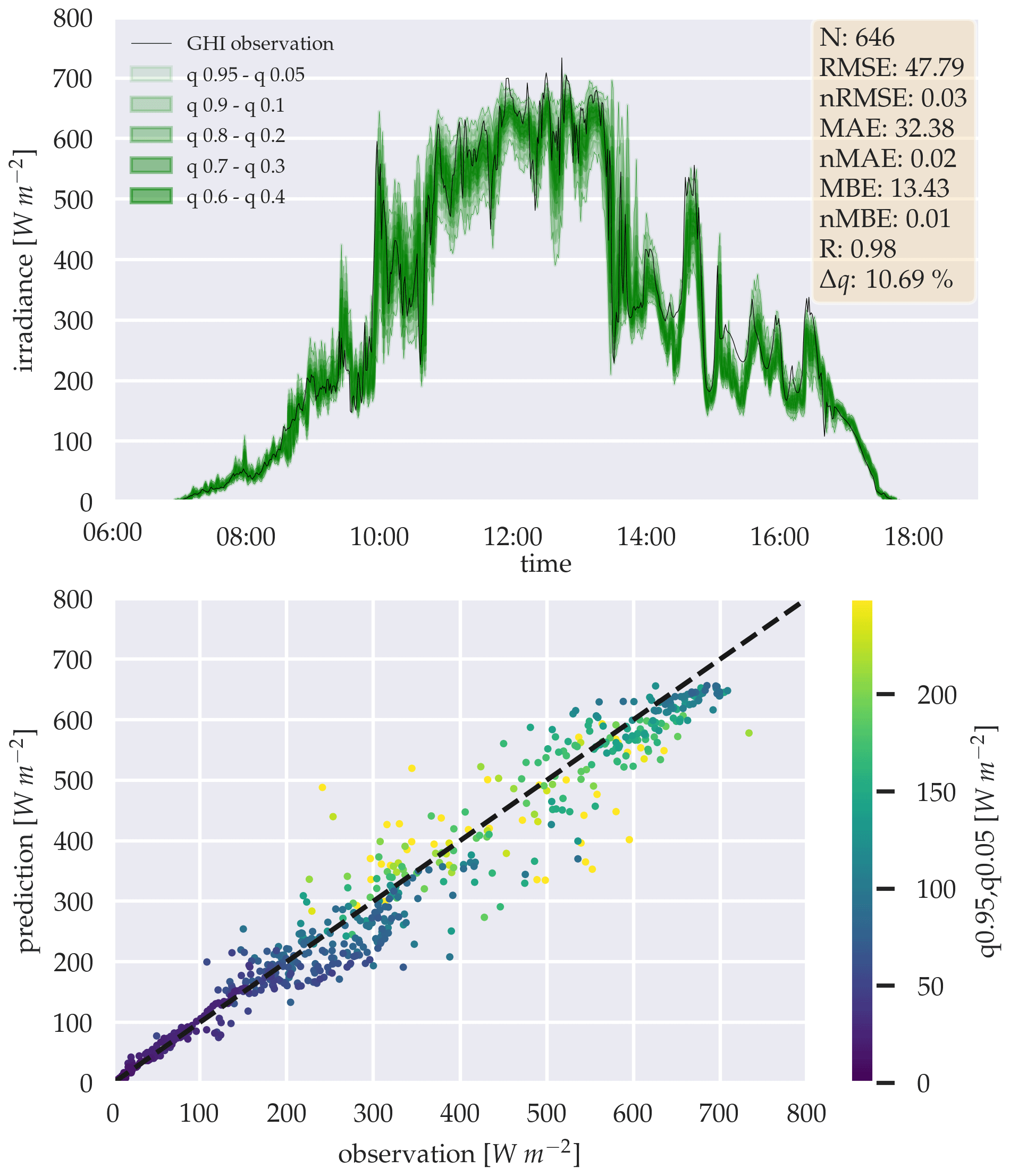
Figure 6Estimation of the GHI for 20 February 2016, using the sinh-arcsinh distribution's quantiles α. The estimations are generated with the probabilistic three-parameter model, and the scatter plot shows the quantile α=0.95 to 0.05.
We then determine its nRMSE and compare it to the nRMSE by the ANN to calculate the forecast skill FS, with
As an example for better illustration, Fig. 6 shows the estimations for 1 d by the probabilistic three-parameter backbone model and the prediction error as a scatter plot with the corresponding quantile range from 0.95 and 0.05 as a color gradient. It is important to note, while a full day would have 1440 data points, given the temporal resolution of the data set of 1 min, the data shown in this study is limited to timings between sunrise and sunset, hence the lower sample size N, as seen in Fig. 6 with N=646. The full data set is evaluated in Sect. 4.1 for the backbone models and Sect. 4.2 for the forecasting models.
A sharpness diagram for the probabilistic three-parameter model is shown in Fig. 7. The diagram provides an estimate of how narrow the quantile ranges are over the population of the forecast distributions. The narrower the quantile ranges and whiskers, the more confident the model is. Note, that this diagram requires that Δq is within an acceptable range. High sharpness with high Δq means, that the model is overconfident, while very low Δq and low sharpness means that the model lacks confidence.
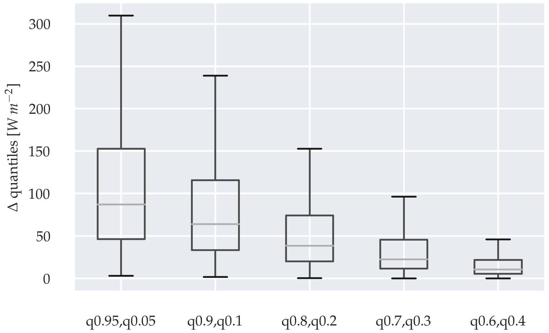
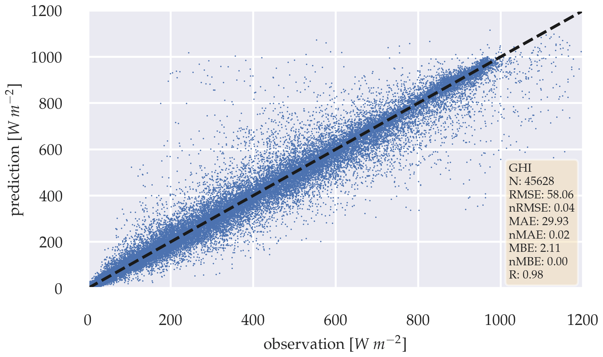
Figure 8Scatter plot between observation and estimation of the deterministic GHI-only model over the whole test data set.
To determine the significance in the model's performance differences, a significance test proposed by Diebold and Mariano (2002) is performed. To determine significance between the distributions means within the sharpness diagram, we use independent trimmed t-test, proposed by Yuen (1974). This test is used to compare distributions with significantly differing variances. To test these variance differences, we perform Levene's test, proposed by Levene (1960). When variance does not differ significantly, Welch's t-test is performed (Welch, 1947). The p-value threshold for rejecting the null hypothesis is <0.05.
We used Tensorflow to design and train our ANN's (Abadi et al., 2015). To pre-process our image data, we used the imageIO and openCV libraries (Silvester et al., 2020; Bradski, 2000). Training was performed on the university's HPC cluster, with nodes consisting of 4 Nvidia HGX-A100 SXM4 GPUs with 80 GB memory connected by 600 GB s−1 NVLink, 2 AMD EPYC 7543 CPU, and 512 GB of system memory. Each node performed the training of two models simultaneously. Inference was performed by using 120 GB system memory and 32 CPU cores, allowing 4 models to be evaluated simultaneously. We summarize our results by using the metrics and statistical tests shown in Sect. 3.4.
4.1 Backbone model
The backbone models show overall good performance in estimating the deterministic and probabilistic irradiance components. Figure 8 shows a scatter plot for the error between the observed and the estimated GHI for the deterministic GHI-only model. The model's error is in a reasonable range considering the error of 2 % by the measurement device (Kern et al., 2023), with an RMSE of 58.06 W m−2 and MAE of 29.93 W m−2. Additionally, the nRMSE of 0.04 and nMAE of 0.02 confirms, that the model produces errors close to the measurement error of the radiometer itself. The MBE of 2.11 W m−2 can be neglected with regards to the measurements error. The observed and estimated GHI correlate closely with R=0.98.
For the simultaneous estimation of the GHI, DNI, and DHI, similar performance can be observed for the GHI estimation, shown in Fig. 9. The RMSE of 59.31 W m−2 and MAE of 30.28 W m−2 shows slightly higher errors, compared to the GHI-only model. MBE can be neglected with 1.43 W m−2, and observation strongly correlates with the estimation (R=0.98). Furthermore, the model can additionally estimate the DNI and DHI with RMSEs of 87.30 and 21.98 W m−2 and MAEs of 42.67 and 12.99 W m−2, respectively. MBE remains low with 0.73 W m−2 for DNI and 0.89 W m−2 for DHI. DNI and DHI estimations correlate closely, with the observation: R=0.97 and 0.98, respectively. However, a one-sided Diebold–Mariano significance test on the GHI estimations of both models showed that the GHI-only model performs significantly better than the three-parameter model with p-value < 0.05 (Diebold and Mariano, 2002).
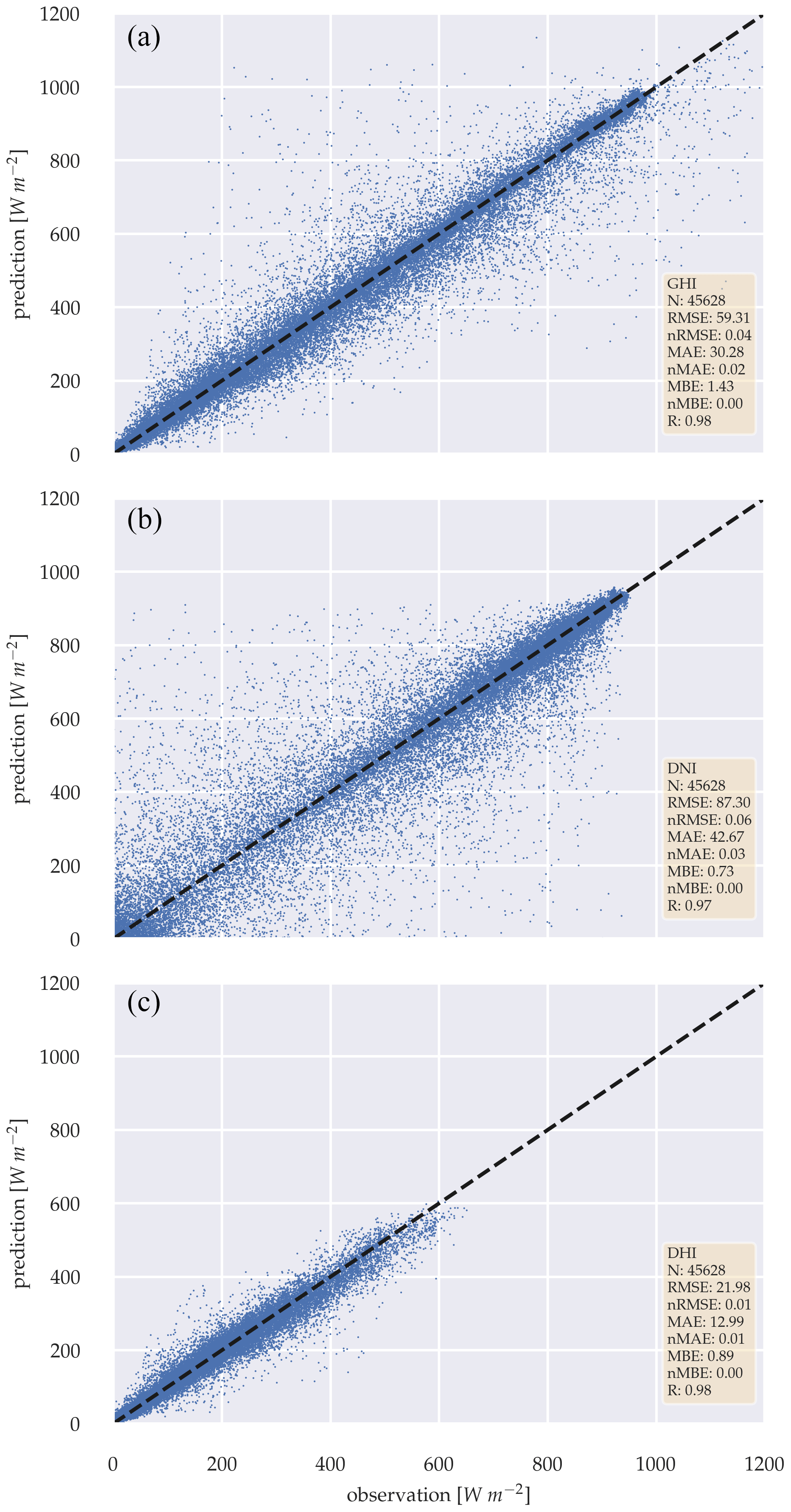
Figure 9Scatter plots between observation and estimation of the deterministic three-parameter model, for GHI (a), DNI (b) and DHI (c) over the whole test data set.
The probabilistic estimation of the GHI results in similar error metrics to those of the deterministic approach, with RMSE 58.36 W m−2, MAE 29.33 W m−2, and MBE of −1.39 W m−2. Figure 10 compares the estimation with the observation as a scatter plot, with Δq0.95,0.05 being colored for each estimation with its magnitude, visualizing the confidence of each estimation. The figure shows that the lower the error, the higher the confidence of the estimation is. When the probabilistic GHI-only model is compared with the deterministic model, a Diebold–Mariano significance test fails to reject the null hypothesis with p-value > 0.05, indicating that there is no significant performance difference between the two methods. A Δq of 13.84 % shows the mean percentage of estimations, which are not inside their respective theoretical quantiles α.
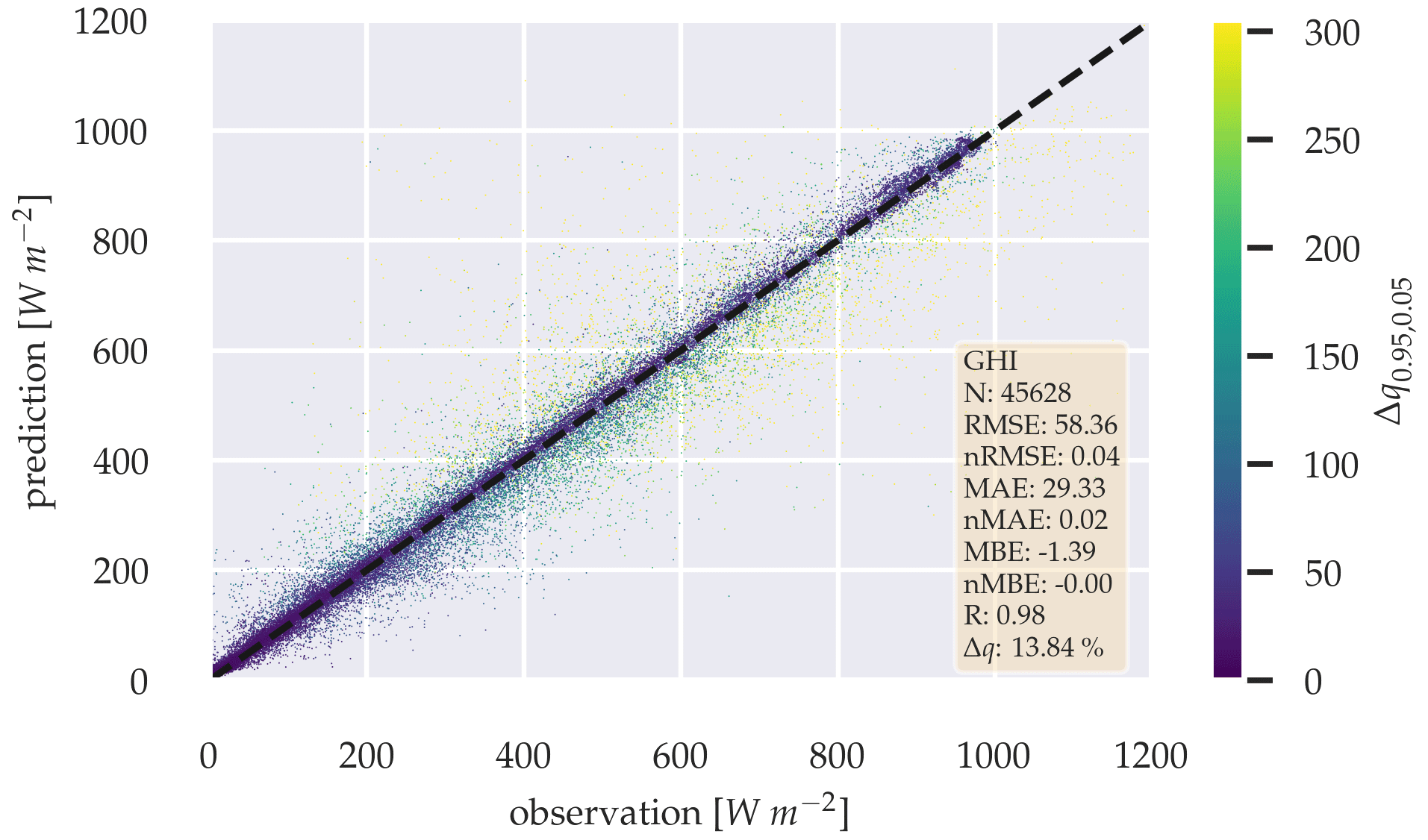
Figure 10Scatter plot between observation and estimation of the probabilistic GHI-only model, with Δq0.95,0.05 being colored according to magnitude over the whole test data set.
Generating three probability distributions for GHI, DNI, and DHI simultaneously shows a more pronounced error increase for all three irradiance components, when compared to the deterministic model counterpart. Figure 11 shows the scatter plots for all three irradiance components. The errors are higher for all irradiance components: RMSE 61.79 W m−2, MAE 29.95 W m−2, and MBE 6.21 W m−2 for GHI; RMSE 99.69 W m−2, MAE 44.27 W m−2, and MBE −1.02 W m−2 for DNI; and RMSE 23.99 W m−2, MAE 12.75 W m−2, and MBE 4.77 W m−2 for DHI. Correlation coefficients range from 0.96 to 0.98. Δqq0.95,0.05 for each GHI estimation increases as the error increases, as observed for the GHI-only model. However, for DNI, this increase is only the case for higher irradiance values, while for DHI only for lower irradiance values. Furthermore, we can observe a decreased Δq of 7.7 %, favoring the three parameter approach in this regard.
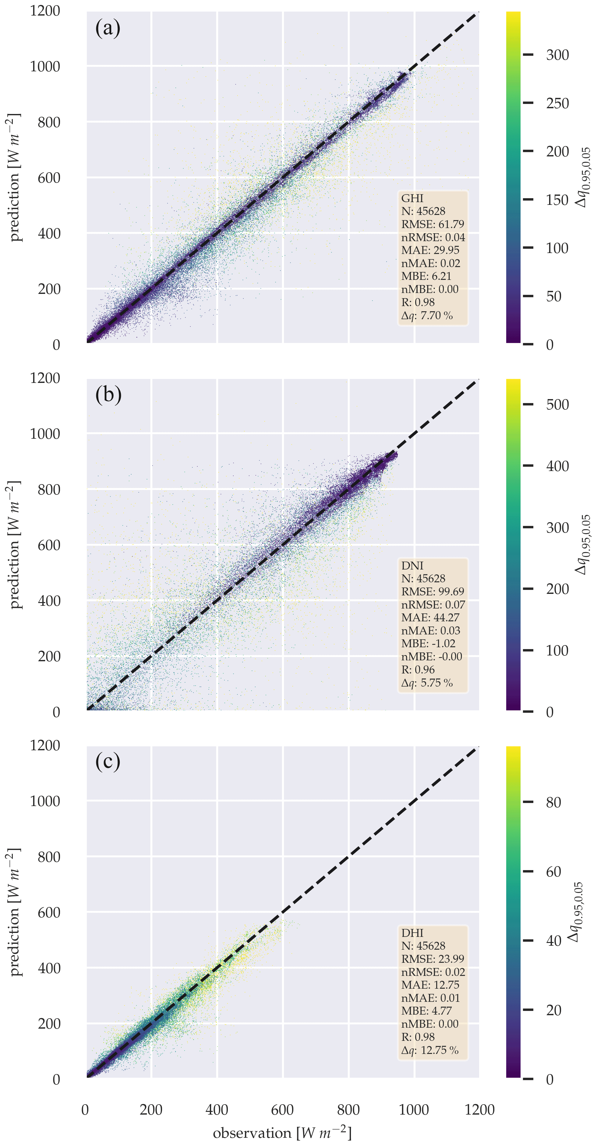
Figure 11Scatter plots between observation and estimation of the probabilistic three-parameter model, for GHI (a), DNI (b) and DHI (c) over the whole test data set.
A Diebold–Mariano significance test confirms that the GHI-only model is significantly better than the three parameter approach with p-value < 0.05. The same results can be observed when testing for significance between the probabilistic and deterministic approaches, confirming that the deterministic three parameter approach performs significantly better than its probabilistic counterpart, with p-value < 0.05.
Further investigations of the probability distributions are illustrated in a sharpness diagram in Fig. 12, grouping the GHI-only model and the components of the three-parameter model into the estimations quantile ranges α. The model shows pronounced uncertainty regarding the estimation of the DNI, with the whiskers range reaching almost half of the possible DNI range for q0.95,0.05. Other radiation components are within more reasonable uncertainties. This difference may be the result of higher gradients compared to the DHI. A comparison between the model's GHI outputs shows an increased sharpness for the GHI-only model. Performing independent trimmed t-test, proposed by Yuen (1974), confirms significance in the difference between the means of the GHI-only model and the GHI of the three-parameter model. This significant increase is the case for each quantile range α, with p-values < 0.05. Furthermore, Levene's test confirms significant differences in variance for all quantile ranges α with p-values < 0.05 (Levene, 1960). The variance reduction observed with the GHI-only model is therefore significant and indicates that the model's confidence fluctuates less, compared to that of the three-parameter model.
Table 3 also indicates that training times are acceptable and inference is below one second. The three-parameter model also shows on both the probabilistic and the deterministic configurations lower training time per epoch and lower inference times.
Table 3Inference and training times for all four backbone configurations. Bold values: arrow up means the higher the better, arrow down means the lower the better and arrow to 0 means the closer to 0 the better.
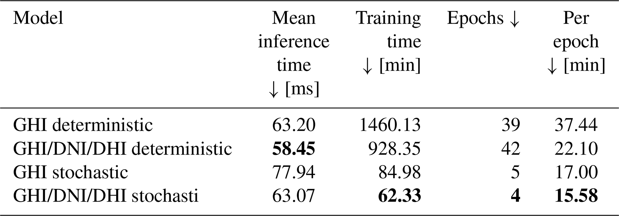
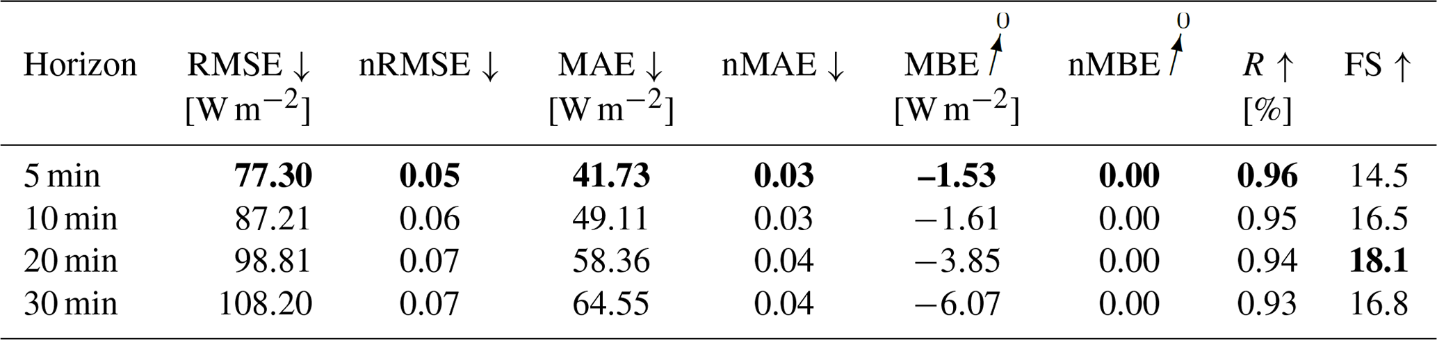
Table 4Evaluation metrics for the GHI-only deterministic forecasting model. Bold values: arrow up means the higher the better, arrow down means the lower the better and arrow to 0 means the closer to 0 the better.
4.2 Forecast model
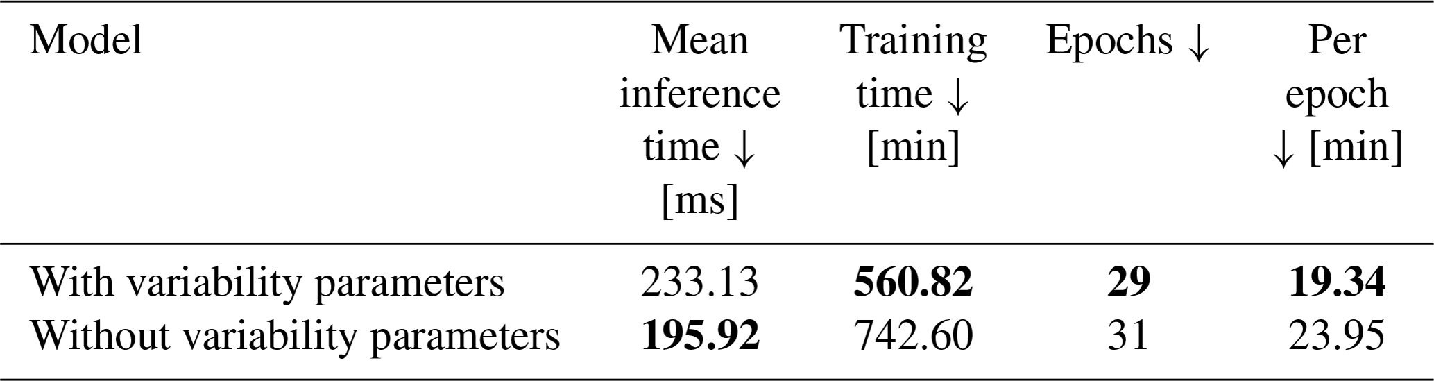
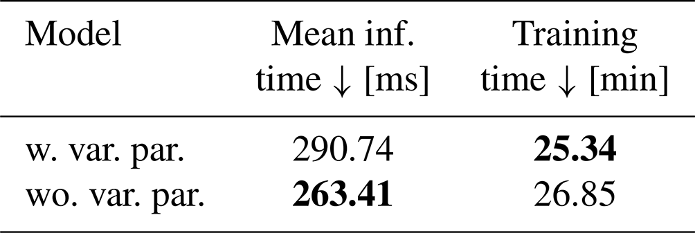
Extending the deterministic estimation task to a forecasting task, as described in Appendix A2, we observe positive skill FS over all forecasting horizons with and without the addition of variability parameters. Training time decreases, compared to the backbone model. This decrease is mainly caused by the decrease of data samples resulting from needing three consecutive ASI image and irradiance data pairs and 1 h of consecutive ASI images for the irradiance estimation. Additionally, data points and images are occasionally missing and additional clear-sky data points are removed. A decrease of training time per epoch can be observed, when adding variability parameters to the training. Also, the model with variability parameters needs fewer epochs to trigger the early stopper. Inference times remain well below one second, although the computation of the variability parameters increases the inference time. Inference and training times are summarized in Table 6.
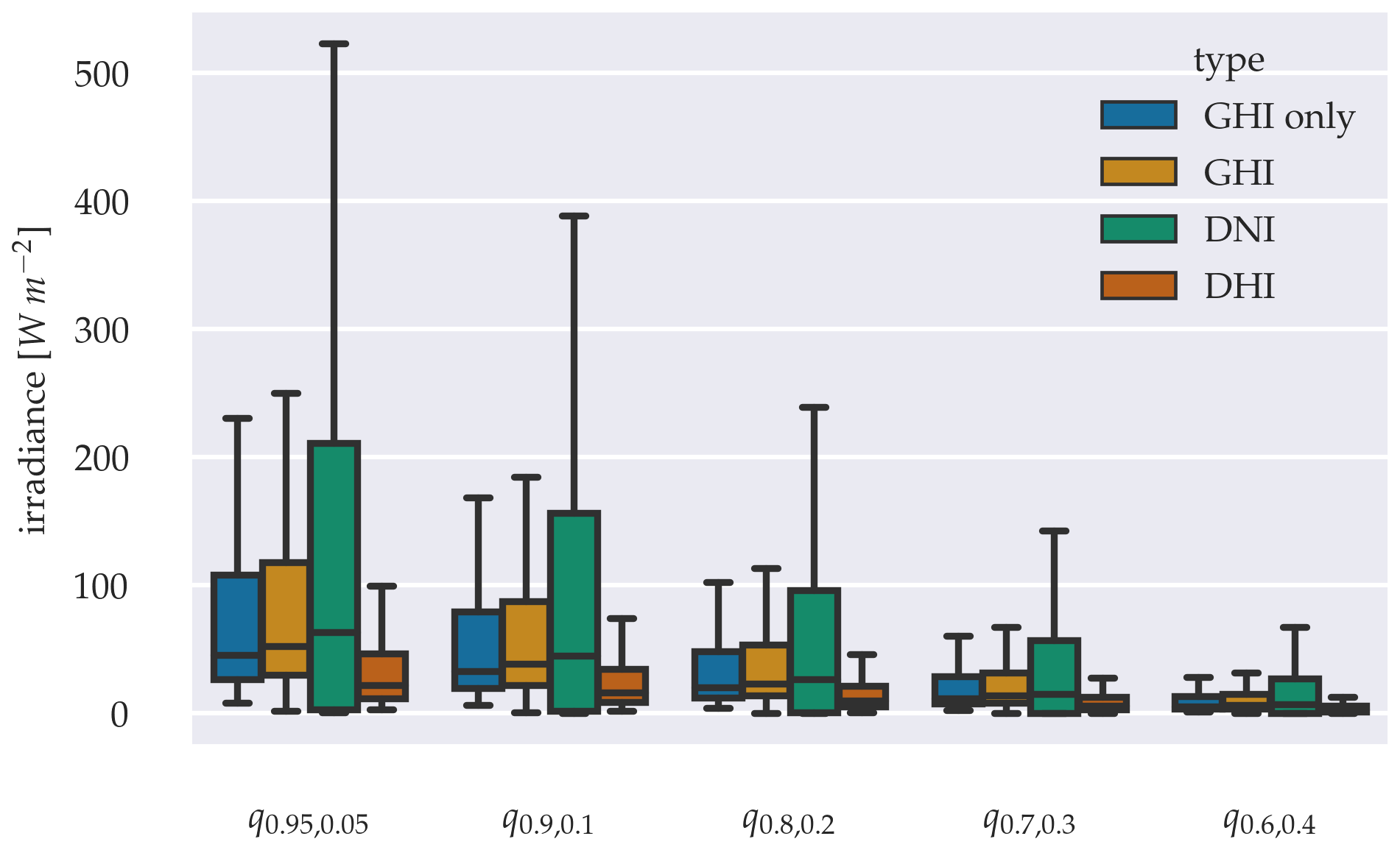
Figure 12Sharpness diagram, grouping GHI-only and three parameter approach into the estimations quantiles ranges α.
For the configuration without variability parameters, errors increase with the forecasting horizon, with RMSE ranging between 77.3 and 108.2 W m−2 and MAE between 41.73 and 64.55 W m−2. RMSE are slightly lower for the horizons 5, 10, and 30 min when adding variability parameters to the model. MAE are higher for all forecasting horizons. A Diebold–Marino significance test fails to reject the null hypothesis with p-value > 0.05, showing that the variability parameters do not significantly impact the model's performance. MBE can be neglected, with −1.53 to −6.07 W m−2. Forecasts highly correlate with observation, with R between 0.96 and 0.93, with forecast skills reaching up to 18.1 %. Similar results can be observed in the configuration with variability parameters. Metrics are summarized in Tables 4 and 5. The metrics confirm that the estimation task can be extended to a forecasting task for different prediction horizons, while maintaining a positive skill score. Figures 13 and 14 illustrate the errors as scatter plots for a 5 min forecasting horizon for both configurations.
Table 5Evaluation metrics for the GHI-only deterministic forecasting model, with variability parameters. Bold values: arrow up means the higher the better, arrow down means the lower the better and arrow to 0 means the closer to 0 the better.
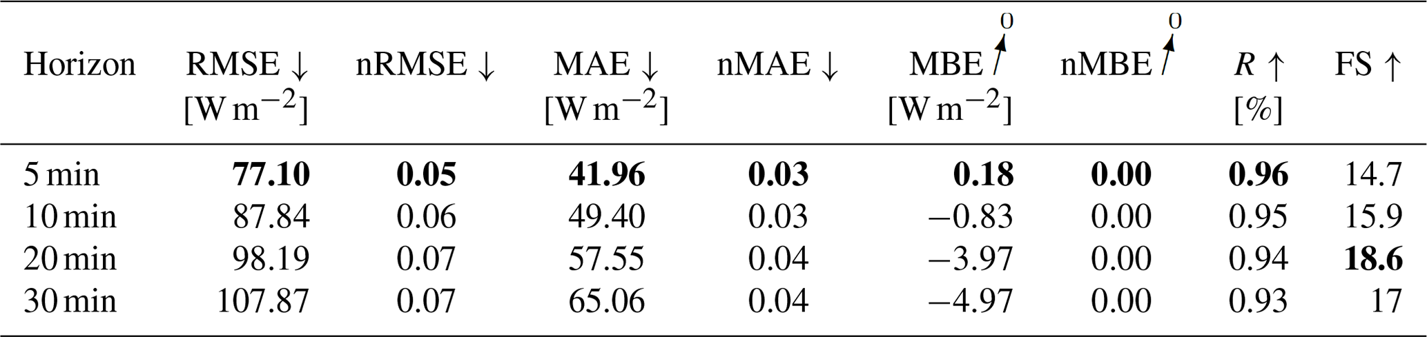
Table 6Inference and training times for the deterministic GHI-only configurations. Bold values: arrow up means the higher the better, arrow down means the lower the better and arrow to 0 means the closer to 0 the better.
When forecasting all three irradiance parameters simultaneously, as shown in Fig. A3, a decrease of training time per epoch can be observed, when adding variability parameters to the training. Also, the number of epochs until triggering the early stopper decreases. Inference time remains, again, well below 1 s, although the calculation of the variability parameters increases the inference time, as with the GHI-only configuration. This increase is mainly caused by the additional calculation of variability parameters derived from estimated DNI values. Inference and training times are summarized in Table 7. A significant performance decrease compared to the GHI-only model can be observed, with p-value < 0.05 in a Diebold-Mariano test. Adding variability parameters to the model does not have any significant impact on the model's performance with p-value > 0.05. Evaluation metrics are summarized in Tables 8 and 9.
Table 7Inference and training times for the deterministic three parameter configurations. Bold values: arrow up means the higher the better, arrow down means the lower the better and arrow to 0 means the closer to 0 the better.
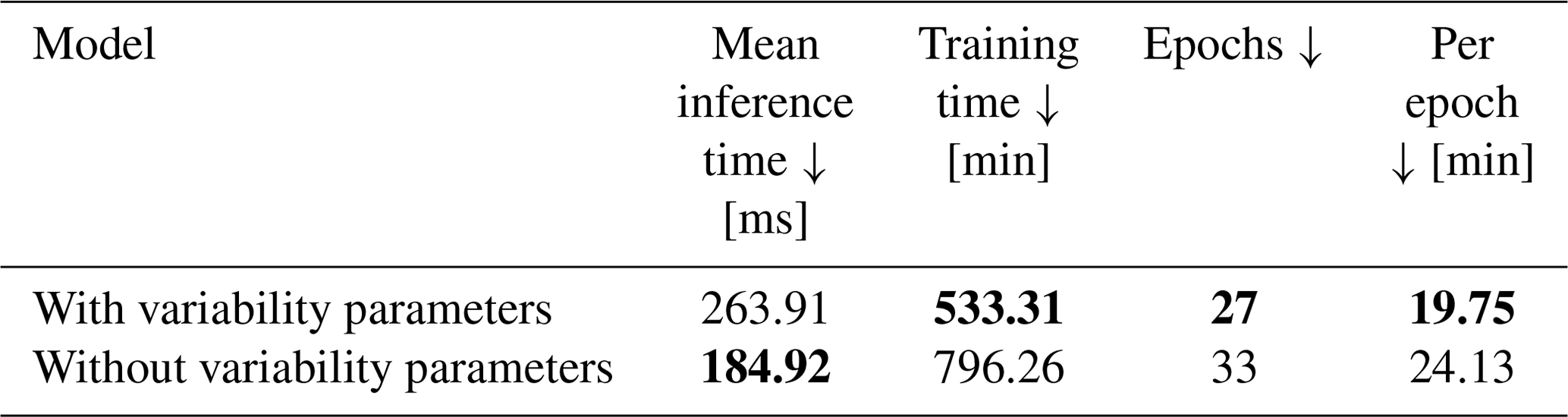

Figure 13Scatter plot between observation and a 5 min forecast of the deterministic GHI-only model, without variability parameters over the whole test data set.
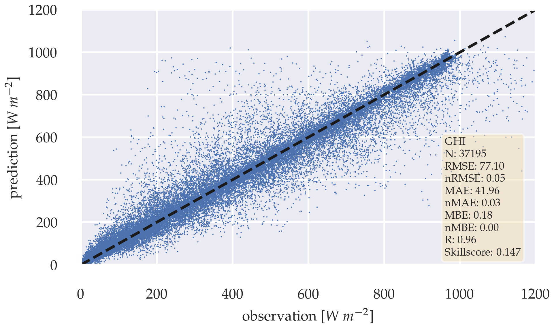
Figure 14Scatter plot between observation and a 5 min forecast of the deterministic GHI-only model, with variability parameters over the whole test data set.
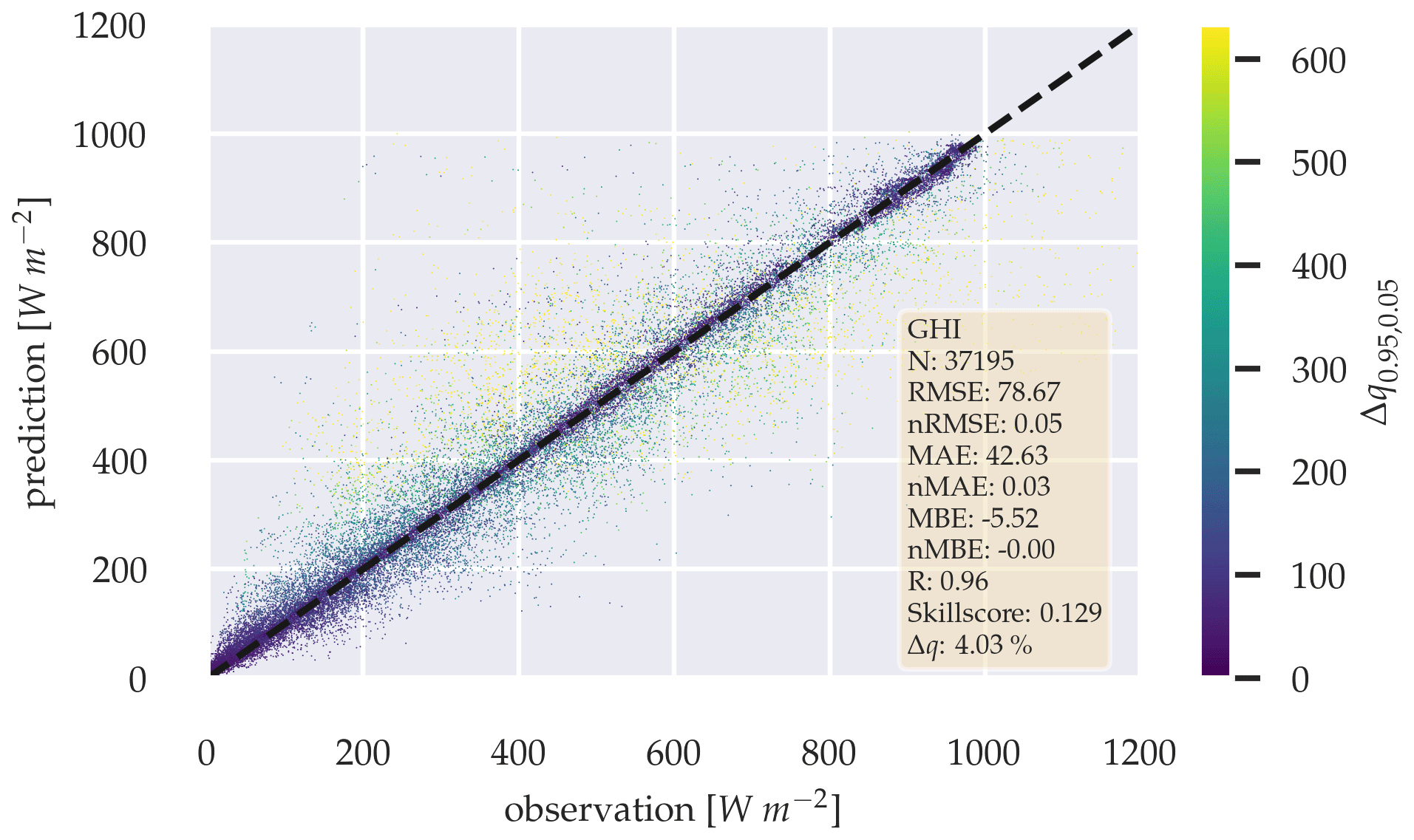
Figure 15Scatter plot between observation and a 5 min forecast of the probabilistic GHI-only model, without variability parameters over the whole test data set.

Figure 16Scatter plot between observation and a 5 min forecast of the probabilistic GHI-only model, with variability parameters over the whole test data set.
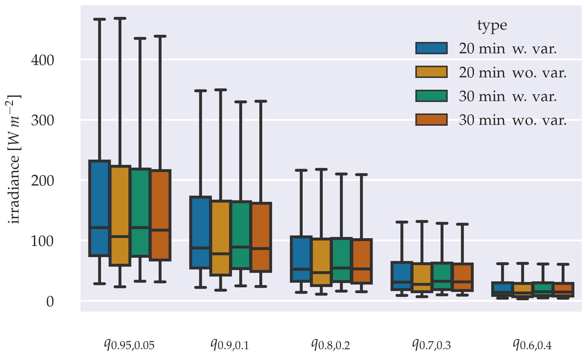
Figure 17Sharpness diagram, grouping the 20 and 30 min forecasting configurations with variability parameter (w. var.) and without variability parameter (wo. var.) into the predictions quantile ranges α.
The probabilistic GHI-only architecture in Fig. A1 shows, that forecasting errors in Table 10 increase significantly, with p-value < 0.05, compared to the deterministic GHI-only model. When variability parameters are added to the model, no significant performance gain can be confirmed from the errors (see Table 11) with p-value > 0.05.
Figures 15 and 16 show the errors of the probabilistic models 5 min forecast as scatter plots. Δq0.95,0.05 is colored according to its error magnitude for each forecast. The plots show, that Δq0.95,0.05 increases with forecast error.
A comparison of Δq for both configurations shows that Δq for forecasting horizons 20 and 30 min are lower when variability parameters are added. The sharpness diagram in Fig. 17 reveals, that all quantiles of the α distribution means are lower in the configuration without variability parameters. The significance of the distribution's mean reductions is confirmed using an independent t-test for distribution pairs with similar variances and independent trimmed t-test for distributions with differing variances, with p-value < 0.05.
Table 8Evaluation metrics for the deterministic forecasting model for all irradiance components. Bold values: arrow up means the higher the better, arrow down means the lower the better and arrow to 0 means the closer to 0 the better.
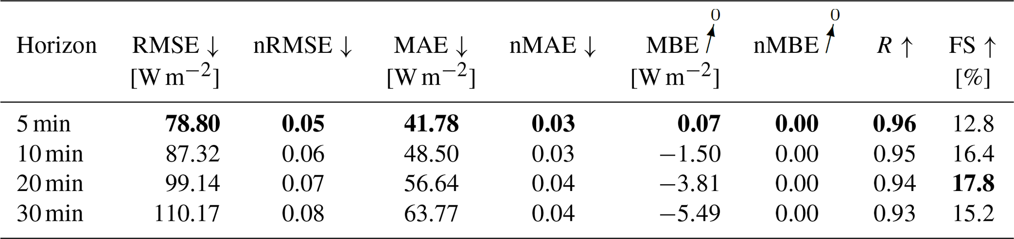
Table 9Evaluation metrics for the deterministic forecasting model for all irradiance components, with variability parameters. Bold values: arrow up means the higher the better, arrow down means the lower the better and arrow to 0 means the closer to 0 the better.
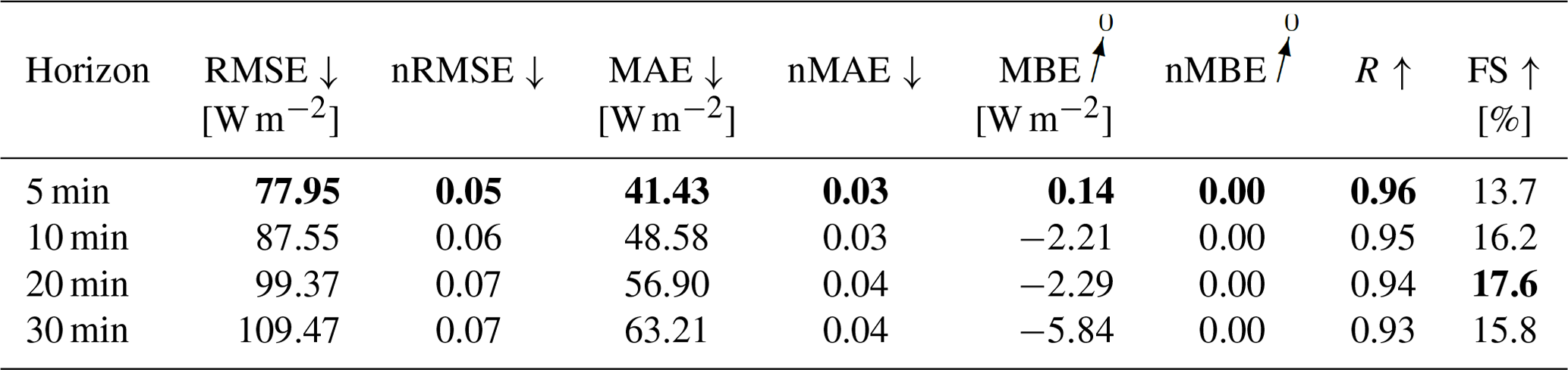
Table 10Evaluation metrics for the GHI-only probabilistic forecasting model. Bold values: arrow up means the higher the better, arrow down means the lower the better and arrow to 0 means the closer to 0 the better.
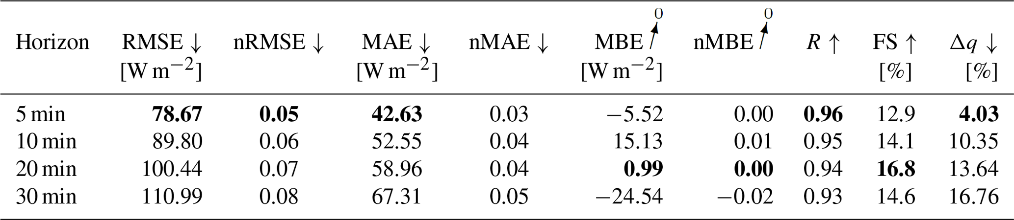
Table 11Evaluation metrics for the GHI-only probabilistic forecasting model, with variability parameters. Bold values: arrow up means the higher the better, arrow down means the lower the better and arrow to 0 means the closer to 0 the better.
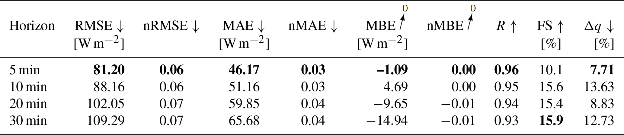
Table 12 shows inference and training times for the probabilistic GHI-only models. The inference time increases but still remains well below one second. The training time per epoch increases and the difference by adding variability parameters decreases.
Table 12Inference and training times for the probabilistic GHI-only configurations. Bold values: arrow up means the higher the better, arrow down means the lower the better and arrow to 0 means the closer to 0 the better.
For further elaboration, example forecasting scenarios and their corresponding image sequences are illustrated and discussed in the Supplement.
In this research, we present a novel approach to training and designing pre-trained neural networks to generate probabilistic solar irradiance forecasts through ASI images. The research questions formulated in Sect. 1 are answered as follows:
-
An estimation of the GHI from ASI images can be performed by exploiting an ImageNet pre-trained ResNet50v2 as feature extractor.
-
With the training data used in our study, the training time of the deterministic backbone models are roughly up to 1 d. The probabilistic backbone models can be trained in even less time with fewer epochs and less training time per epoch. Using all three irradiance components for the estimation task, seems to decrease the training time per epoch. The deterministic forecasting models can be trained in well below 1 d. Adding variability parameters has been shown to reduce, both epoch count and training time per epoch. The probabilistic forecasting models train much faster with training times below half an hour. The training speed gains observed for adding variability parameters are less pronounced.
-
Adding the DNI and DHI to the estimation task, significantly increases the error of the GHI estimation. This is true for both the deterministic and probabilistic model and an equal loss weighting for all three irradiance components.
-
It is possible to generate irradiance probability distributions of the GHI without a significant error increase, compared to the deterministic model.
-
Forecasts with positive skill are possible for deterministic and probabilistic GHI forecasts of up to 30 min. Adding the DNI and DHI with equal loss weighting significantly increases the error of the GHI forecast but a positive skill score is maintained. The forecast skill of the GHI-only model decreases significantly when transitioning to a probabilistic forecasting task, but offers additional information about the model's confidence.
-
Overall, the set of variability parameters proposed by Schroedter-Homscheidt et al. (2018) generally do not have a significant impact on the model's forecasting performance.
-
Inference times remain below one second, ranging from 184.92 to 290.74 ms for the forecasting models and 63.07 to 77.94 ms for the backbone models.
The empirical coverage of the distributions Δqα by the probabilistic forecasting model might be reduced by utilizing calibration techniques on the neural network, such as defining Δqα as a loss function. Quantifying the sharpness diagrams properly might also be a good method to be incorporated within the loss function. The Brier-Score, proposed by Brier (1950), and/or combining these loss functions could also be an option to calibrate the model properly and thus maintain good empirical coverage and high sharpness.
The observed training time reduction through the set of variability parameters proposed by Schroedter-Homscheidt et al. (2018), shows that meteorological findings should not only be considered for assisting ANNs in performance increase but also for reducing the ANNs training time. Additionally, predicting variability parameters rather than irradiance values can illuminate whether an ANN can extract such information from the input image sequence and how it does so.
Regarding training time, the same is true for adding the DNI and DHI to the estimation task. While the maximum reported training time of roughly 1 d might not be a long period for training ANNs, this might be a critical factor when training on a larger set of ASI images and irradiance data from all over the world. Furthermore, varying the loss weights among the GHI, DNI and DHI in the three-parameter model could also lead to different results, instead of treating all three parameters equally. This needs to be evaluated in future work.
Modifying the architecture of the LSTM and Dense layers for the forecast model could potentially enhance performance in predicting the target feature vector based on the current and past feature vectors. Experimenting with different configurations and sizes of these layers may reveal valuable insights into efficiency improvements and more accurate predictions. This approach involves exploring variations in layer parameters, such as the number of units in LSTM layers or the activation functions in Dense layers, to optimize the model's ability to learn and generalize from temporal data sequences. Additionally, incorporating a broader and more detailed series of input images could further refine the model's capacity to effectively learn and extract meaningful patterns from temporal data sequences.
Pothineni et al. (2019) also reported an increase in accuracy of forecasts when training data from different geographical locations with differing atmospheric conditions are used. While this performance increase was only confirmed on deterministic forecasts, it is plausible that the same is the case for probabilistic forecasts. Therefore, we are currently gathering ASI images and irradiance data from Ghana within the framework of the EnerSHelF project to test our findings on a more unique data set (Meilinger and Bender, 2023; Yousif et al., 2022). While this study confirmed the possibility to use an ImageNet pre-trained ANN models for our application, it should also be possible to use the trained models as pre-trained backbones on more unique and sparse data sets as a transfer learning technique. The method also needs a cross-validation on different sites, to determine the effectiveness of using the ASI as radiometer during deployment.
It is also important to emphasize that this study filtered out most clear-sky situations from the dataset to focus on non-clear-sky conditions. Despite the ability of our model to predict clear-sky situations, as shown in the supplementary material, predicting such clear-sky situations would be a proper approach to differentiate situations where more conservative methods are more suitable for predicting the irradiance. One approach would be using our method to replace the labels with a binary clear-sky label to train the model on a binary cross-entropy loss function. Labeling the images as clear-sky can be done via the clear-sky detection method used in this study. We have performed a preliminary study, using a pre-trained ResNet50v2 classifier and modifying its output vector to output two instead of 1000 classes. These two classes represent clear-sky and non-clear-sky. The general principle is shown in Fig. A4. After training this model, we achieve an accuracy of 93.2 %. Extending the model to a forecasting model, similar to the approach proposed in this study, we achieve a binary accuracy of 93.3 % for a 5 min forecasting horizon, 93.2 % for a 10 min forecasting horizon, 91.6 % for a 20 min forecasting horizon and 90.6 % for a 30 min forecasting horizon. The architecture is shown in Fig. A5.
Leveraging the method to segment the ASI images through a U-Net to determine the presence of clouds, as proposed by Fabel et al. (2022), can also be a proper approach to differentiate between clear-sky and non-clear-sky conditions and apply proper labeling. Using other clear-sky products to label the data, like the Copernicus Atmosphere Monitoring Service McClear model (Lefèvre et al., 2013), can also be considered.
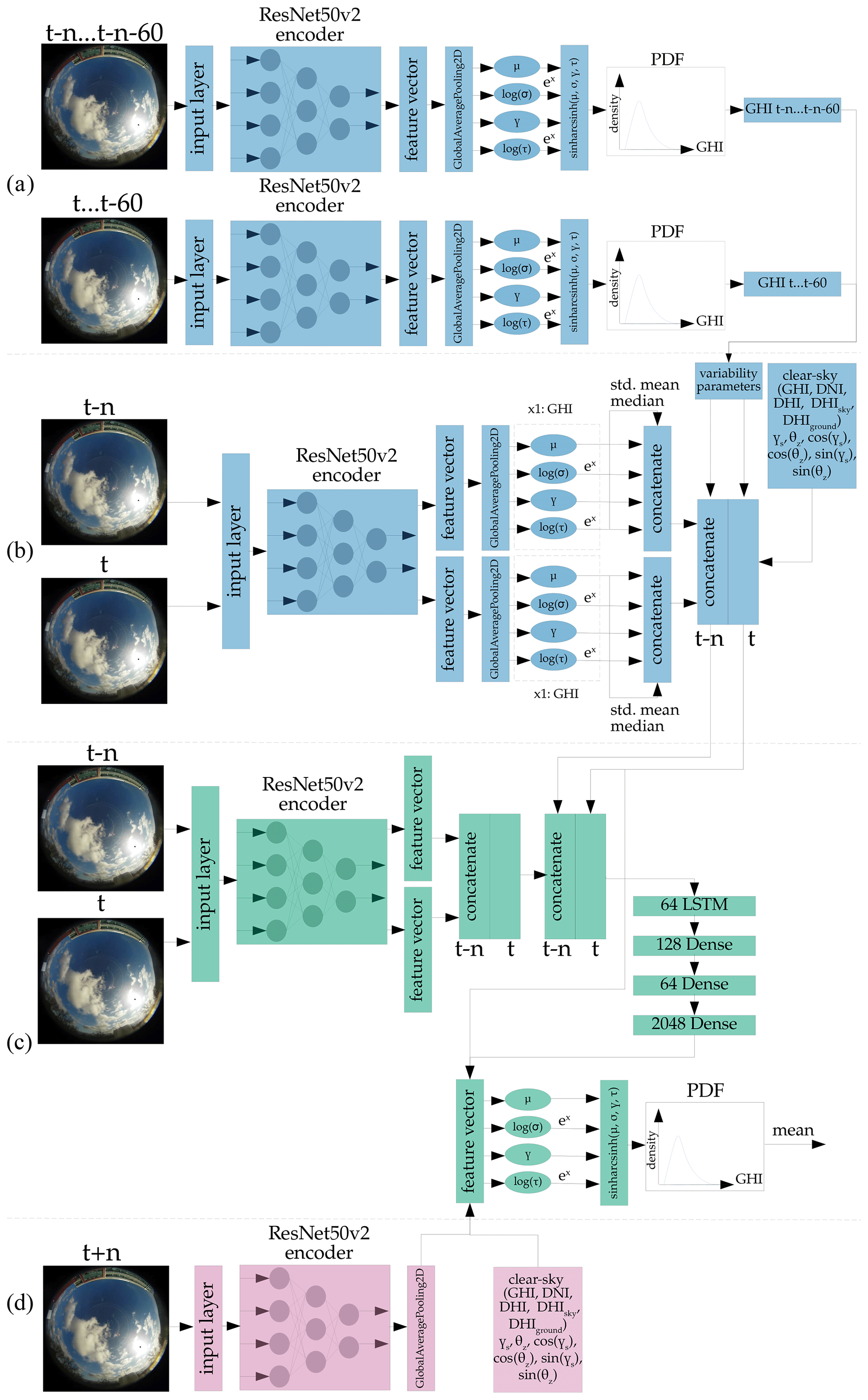
Figure A1Architecture of the probabilistic forecast model, forecasting the probability distribution of the GHI. Blue – not trained, but part of training; green – trained; pink – not trained, and not part of training.

Figure A2Architecture of the deterministic forecast model, forecasting the GHI. Blue – not trained, but part of training; green – trained; pink – not trained, and not part of training.
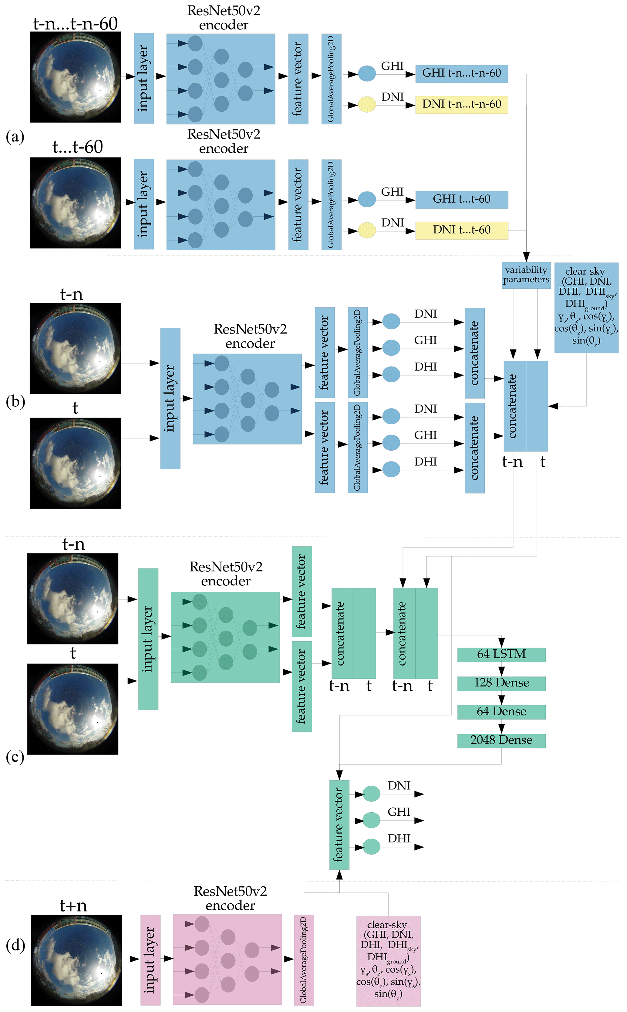
Figure A3Architecture of the deterministic forecast model, forecasting the GHI, DNI, and DHI simultaneously. Blue – not trained, but part of training; green – trained; pink – not trained and not part of training; yellow – not trained, part of training, and optional.
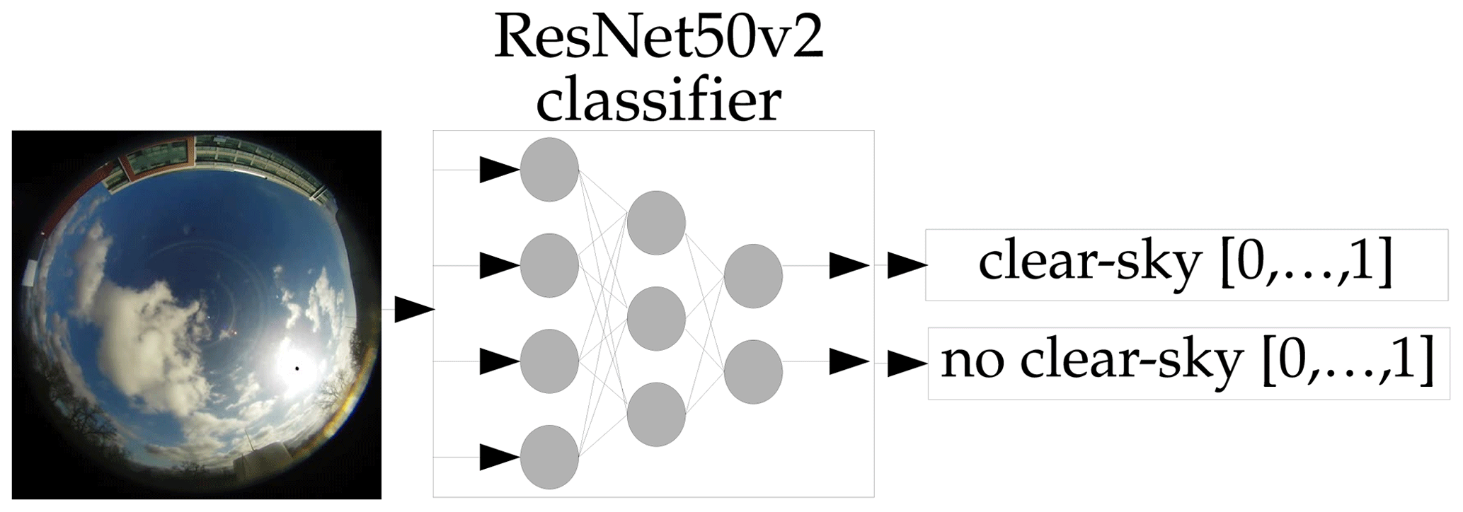
Figure A4Principle of the backbone clear-sky classification model, based on a ResNet50v2 classifier. The output vector has the dimension of 2, instead of the original 1000. The first output is for clear-sky (1 = True, 0 = False). The second output is for non-clear-sky (1 = True, 0 = False). The model can output values between 1 and 0, giving information about the models confidence.
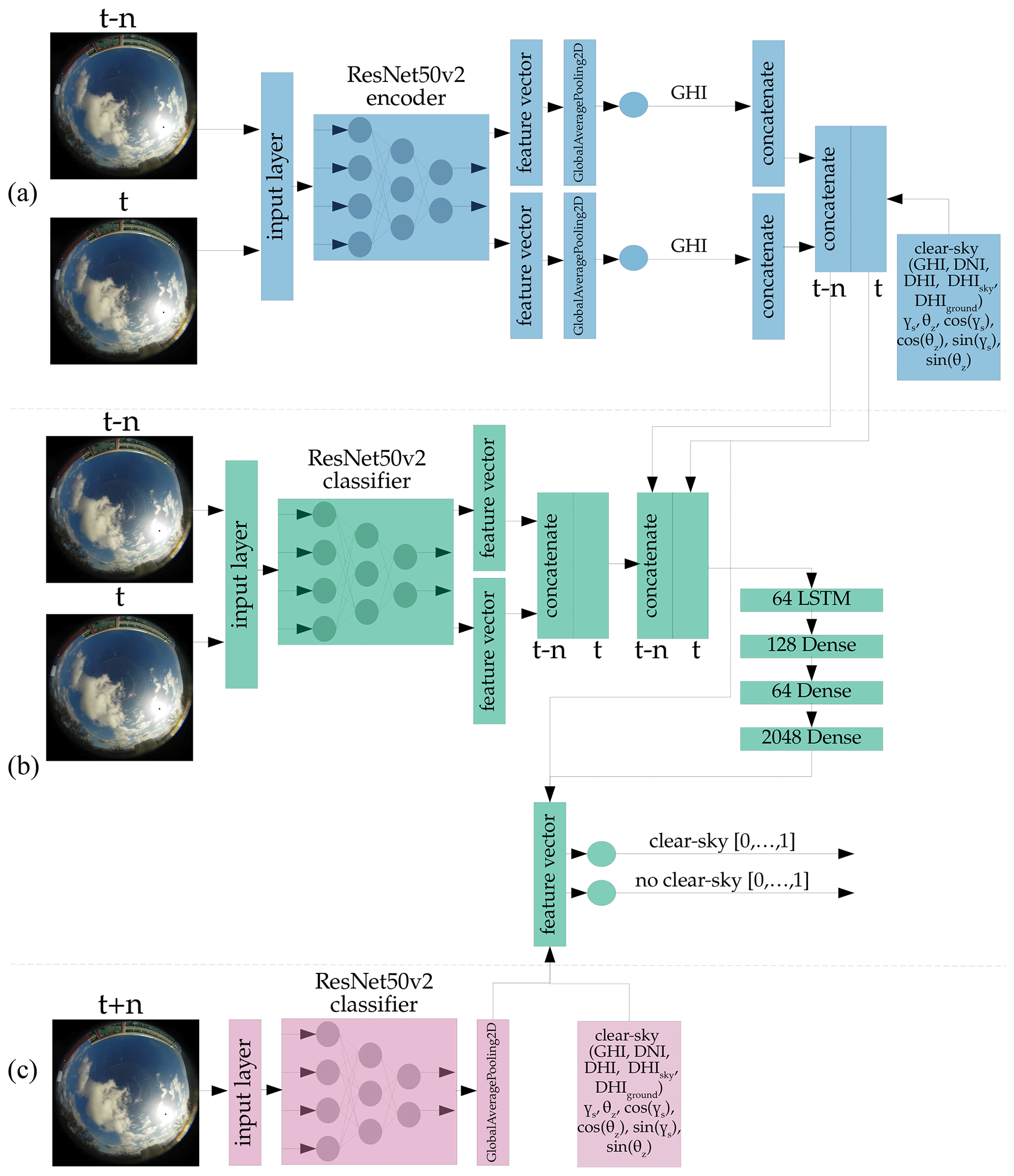
Figure A5Architecture of a probabilistic clear-sky forecast model. Blue – not trained, but part of training; green – trained; pink – not trained and not part of training; yellow - not trained, part of training, and optional. (a) uses the ResNet50v2 backbone for estimating the current and past GHI, as in Fig. A2. (b) and (c) use the ResNet50v2 classifier in Fig. A4.
The Tensorflow code relevant for the probabilistic output layers is referenced in Barnes et al. (2021) (https://doi.org/10.48550/ARXIV.2109.07250), specifically in Appendices C–E. The remaining code adheres to standard Tensorflow conventions and does not claim to be original in design. Essential configuration parameters are detailed within the paper. For further inquiries, requests or assistance for the code, please contact the corresponding author.
The images from the All-Sky Imager (ASI) and the associated irradiance values featured in this study are available for download at https://doi.org/10.5281/zenodo.2826938 (Carreira Pedro et al., 2019).
The supplement related to this article is available online at: https://doi.org/10.5194/asr-20-129-2024-supplement.
Conceptualization, SC, SH, SM; methodology, SC, SH, SM; software, SC; validation, SC; formal analysis, SC, SH, SM; investigation, SC; resources, SC, SM, SH; data curation, SC; writing – original draft preparation, SC; writing – review and editing, SC, SH, SM; visualization, SC; supervision, SH, SM; project administration, SM; funding acquisition, SM.
The contact author has declared that none of the authors has any competing interests.
This article is part of the special issue “EMS Annual Meeting: European Conference for Applied Meteorology and Climatology 2022”. It is a result of the EMS Annual Meeting: European Conference for Applied Meteorology and Climatology 2022, Bonn, Germany, 4–9 September 2022. The corresponding presentation was part of session OSA1.1: Forecasting, nowcasting and warning systems.
Publisher's note: Copernicus Publications remains neutral with regard to jurisdictional claims made in the text, published maps, institutional affiliations, or any other geographical representation in this paper. While Copernicus Publications makes every effort to include appropriate place names, the final responsibility lies with the authors.
This research has been supported by the Bundesministerium für Bildung und Forschung (grant no. 03SF0567A-G).
This paper was edited by Maurice Schmeits and reviewed by two anonymous referees.
Abadi, M., Agarwal, A., Barham, P., Brevdo, E., Chen, Z., Citro, C., Corrado, G. S., Davis, A., Dean, J., Devin, M., Ghemawat, S., Goodfellow, I., Harp, A., Irving, G., Isard, M., Jia, Y., Jozefowicz, R., Kaiser, L., Kudlur, M., Levenberg, J., Mané, D., Monga, R., Moore, S., Murray, D., Olah, C., Schuster, M., Shlens, J., Steiner, B., Sutskever, I., Talwar, K., Tucker, P., Vanhoucke, V., Vasudevan, V., Viégas, F., Vinyals, O., Warden, P., Wattenberg, M., Wicke, M., Yu, Y., and Zheng, X.: TensorFlow: Large-Scale Machine Learning on Heterogeneous Systems, http://tensorflow.org/ (last access: 26 December 2023), 2015. a, b
Amos, D. E.: Algorithm 644: A Portable Package for Bessel Functions of a Complex Argument and Nonnegative Order, ACM Trans. Math. Softw., 12, 265–273, https://doi.org/10.1145/7921.214331, 1986. a
Barnes, E. A., Barnes, R. J., and Gordillo, N.: Adding Uncertainty to Neural Network Regression Tasks in the Geosciences, arXiv [preprint], https://doi.org/10.48550/ARXIV.2109.07250, 2021. a, b, c, d, e
Bouktif, S., Fiaz, A., Ouni, A., and Serhani, M.: Optimal Deep Learning LSTM Model for Electric Load Forecasting using Feature Selection and Genetic Algorithm: Comparison with Machine Learning Approaches, Energies, 11, 1636, https://doi.org/10.3390/en11071636, 2018. a
Bozkurt, Ö. Ö., Biricik, G., and Taysi, Z. C.: Artificial neural network and SARIMA based models for power load forecasting in Turkish electricity market, PLOS ONE, 12, 1–24, https://doi.org/10.1371/journal.pone.0175915, 2017. a
Bradski, G.: The OpenCV Library, Dr. Dobb's Journal of Software Tools, https://opencv.org/ (last access: 26 December 2023), 2000. a
Bremnes, J. B.: Probabilistic Forecasts of Precipitation in Terms of Quantiles Using NWP Model Output, Mon. Weather Rev., 132, 338–347, https://doi.org/10.1175/1520-0493(2004)132<0338:PFOPIT>2.0.CO;2, 2004. a
Brier, G. W.: Verification Of Forecasts Expressed In Terms Of Probabilty, Mon. Weather Rev., 78, 1–3, https://doi.org/10.1175/1520-0493(1950)078<0001:VOFEIT>2.0.CO;2, 1950. a
Brown, T. B., Mann, B., Ryder, N., Subbiah, M., Kaplan, J., Dhariwal, P., Neelakantan, A., Shyam, P., Sastry, G., Askell, A., Agarwal, S., Herbert-Voss, A., Krueger, G., Henighan, T., Child, R., Ramesh, A., Ziegler, D. M., Wu, J., Winter, C., Hesse, C., Chen, M., Sigler, E., Litwin, M., Gray, S., Chess, B., Clark, J., Berner, C., McCandlish, S., Radford, A., Sutskever, I., and Amodei, D.: Language Models are Few-Shot Learners, arXiv [preprint], https://doi.org/10.48550/arXiv.2005.14165, 2020. a
Bruno, S., Dellino, G., La Scala, M., and Meloni, C.: A Microforecasting Module for Energy Management in Residential and Tertiary Buildings, Energies, 12, 1006, https://doi.org/10.3390/en12061006, 2019. a
Carreira Pedro, H., Larson, D., and Coimbra, C.: A comprehensive dataset for the accelerated development and benchmarking of solar forecasting methods (Version V1) [Data set], Zenodo [data set], https://doi.org/10.5281/zenodo.2826939, 2019. a
Chaaraoui, S., Bebber, M., Meilinger, S., Rummeny, S., Schneiders, T., Sawadogo, W., and Kunstmann, H.: Day-Ahead Electric Load Forecast for a Ghanaian Health Facility Using Different Algorithms, Energies, 14, 409, https://doi.org/10.3390/en14020409, 2021. a
Chaaraoui, S., Houben, S., and Meilinger, S.: End to End Global Horizontal Irradiance Estimation Through Pre-trained Deep Learning Models Using All-Sky-Images, in: EMS Annual Meeting 2022, 4–9 September 2022, Bonn, Germany, https://doi.org/10.5194/ems2022-505, 2022. a
Coimbra, C. F., Kleissl, J., and Marquez, R.: Chapter 8 – Overview of Solar-Forecasting Methods and a Metric for Accuracy Evaluation, in: Solar Energy Forecasting and Resource Assessment, edited by: Kleissl, J., Academic Press, Boston, 171–194, ISBN 978-0-12-397177-7, https://doi.org/10.1016/B978-0-12-397177-7.00008-5, 2013. a
Deng, J., Dong, W., Socher, R., Li, L.-J., Li, K., and Fei-Fei, L.: ImageNet: A large-scale hierarchical image database, in: 2009 IEEE Conference on Computer Vision and Pattern Recognition, 20–25 June 2009, Miami, FL, USA, 248–255, https://doi.org/10.1109/CVPR.2009.5206848, 2009. a
Devlin, J., Chang, M.-W., Lee, K., and Toutanova, K.: BERT: Pre-training of Deep Bidirectional Transformers for Language Understanding, arXiv [preprint], https://doi.org/10.48550/ARXIV.1810.04805, 2019. a
Diagne, H. M., Lauret, P., and David, M.: Solar irradiation forecasting: state-of-the-art and proposition for future developments for small-scale insular grids, in: WREF 2012 – World Renewable Energy Forum, Denver, USA, https://hal.archives-ouvertes.fr/hal-00918150, 2012. a
Diebold, F. X. and Mariano, R. S.: Comparing Predictive Accuracy, J. Business Econ. Stat., 20, 134–144, https://doi.org/10.1198/073500102753410444, 2002. a, b
Dongol, D.: Development and implementation of model predictive control for a photovoltaic battery system, PhD thesis, Universität Freiburg, Freiburg, https://doi.org/10.6094/UNIFR/149249, 2019. a, b
Du, H., He, Y., and Jin, T.: Transfer Learning for Human Activities Classification Using Micro-Doppler Spectrograms, in: 2018 IEEE International Conference on Computational Electromagnetics (ICCEM), 26–28 March 2018, Chengdu, China, 1–3, https://doi.org/10.1109/COMPEM.2018.8496654, 2018. a
Fabel, Y., Nouri, B., Wilbert, S., Blum, N., Triebel, R., Hasenbalg, M., Kuhn, P., Zarzalejo, L. F., and Pitz-Paal, R.: Applying self-supervised learning for semantic cloud segmentation of all-sky images, Atmos. Meas. Tech., 15, 797–809, https://doi.org/10.5194/amt-15-797-2022, 2022. a, b
Feng, C., Zhang, W., Hodge, B.-M., and Zhang, Y.: Occlusion-perturbed Deep Learning for Probabilistic Solar Forecasting via Sky Images, in: 2022 IEEE Power I & Energy Society General Meeting (PESGM), 17–21 July 2022, Denver, CO, USA, 1–5, https://doi.org/10.1109/PESGM48719.2022.9917222, 2022. a, b, c
Ferreira, C. A., Melo, T., Sousa, P., Meyer, M. I., Shakibapour, E., Costa, P., and Campilho, A.: Classification of Breast Cancer Histology Images Through Transfer Learning Using a Pre-trained Inception Resnet V2, in: Image Analysis and Recognition, Springer International Publishing, 763–770, ISBN 978-3-319-93000-8, https://doi.org/10.1007/978-3-319-93000-8_86, 2018. a
Gneiting, T., Balabdaoui, F., and Raftery, A. E.: Probabilistic forecasts, calibration and sharpness, J. Roy. Stat. Soc. B, 69, 243–268, https://doi.org/10.1111/j.1467-9868.2007.00587.x, 2007. a
Hasenbalg, M., Kuhn, P., Wilbert, S., Nouri, B., and Kazantzidis, A.: Benchmarking of six cloud segmentation algorithms for ground-based all-sky imagers, Solar Energy, 201, 596–614, https://doi.org/10.1016/j.solener.2020.02.042, 2020. a
He, K., Zhang, X., Ren, S., and Sun, J.: Deep Residual Learning for Image Recognition, arXiv [prepint], https://doi.org/10.48550/ARXIV.1512.03385, 2015. a
He, K., Zhang, X., Ren, S., and Sun, J.: Identity Mappings in Deep Residual Networks, in: Computer Vision – ECCV 2016, Springer International Publishing, Cham, 630–645, https://doi.org/10.48550/ARXIV.1603.05027, 2016. a
Howard, A. G., Zhu, M., Chen, B., Kalenichenko, D., Wang, W., Weyand, T., Andreetto, M., and Adam, H.: MobileNets: Efficient Convolutional Neural Networks for Mobile Vision Applications, arXiv [preprint], https://doi.org/10.48550/arXiv.1704.04861, 2017. a
Ineichen, P. and Perez, R.: A new airmass independent formulation for the Linke turbidity coefficient, Solar Energy, 73, 151–157, https://doi.org/10.1016/S0038-092X(02)00045-2, 2002. a
Jones, M. C. and Pewsey, A.: Sinh-arcsinh distributions, Biometrika, 96, 761–780, https://doi.org/10.1093/biomet/asp053, 2009. a, b
Jung, S.: Variabilität der solaren Einstrahlung in 1-Minuten aufgelösten Strahlungszeitserien, PhD thesis, https://elib.dlr.de/100762/ (last access: 26 December 2023), 2015. a
Kern, E. C., Augustyn, J., and Bing, J.: RSR2 Rotating Shadowband Radiometer Product Brochure, Campbell Scientific Southeast Asia, https://s.campbellsci.com/documents/au/product-brochures/b_rsr2.pdf (last access: 26 December 2023), 2023. a
Kober, K., Craig, G. C., Keil, C., and Dörnbrack, A.: Blending a probabilistic nowcasting method with a high-resolution numerical weather prediction ensemble for convective precipitation forecasts, Q. J. Roy. Meteorol. Soc., 138, 755–768, https://doi.org/10.1002/qj.939, 2012. a
Kraas, B., Schroedter-Homscheidt, M., and Madlener, R.: Economic merits of a state-of-the-art concentrating solar power forecasting system for participation in the Spanish electricity market, Solar Energy, 93, 244–255, https://doi.org/10.1016/j.solener.2013.04.012, 2013. a
Krizhevsky, A., Sutskever, I., and Hinton, G. E.: Imagenet classification with deep convolutional neural networks, Adv. Neural Inf. Process. Syst., 25, 1097–1105, 2012. a
Lefèvre, M., Oumbe, A., Blanc, P., Espinar, B., Gschwind, B., Qu, Z., Wald, L., Schroedter-Homscheidt, M., Hoyer-Klick, C., Arola, A., Benedetti, A., Kaiser, J. W., and Morcrette, J.-J.: McClear: a new model estimating downwelling solar radiation at ground level in clear-sky conditions, Atmos. Meas. Tech., 6, 2403–2418, https://doi.org/10.5194/amt-6-2403-2013, 2013. a
Levene, H.: Robust tests for equality of variances, Contributions to Probability and Statistics: Essays in Honor of Harold Hotelling, Stanford University Press, Palo Alto, 278–292, ISBN 0-8047-0596-8, 1960. a, b
Liu, Z., Mao, H., Wu, C.-Y., Feichtenhofer, C., Darrell, T., and Xie, S.: A ConvNet for the 2020s, arXiv [preprint], https://doi.org/10.48550/arXiv.2201.03545, 2022. a
Maheri, A.: Multi-objective design optimisation of standalone hybrid wind-PV-diesel systems under uncertainties, Renew. Energy, 66, 650–661, https://doi.org/10.1016/j.renene.2014.01.009, 2014. a
Maitanova, N., Telle, J.-S., Hanke, B., Grottke, M., Schmidt, T., Maydell, K. V., and Agert, C.: A Machine Learning Approach to Low-Cost Photovoltaic Power Prediction Based on Publicly Available Weather Reports, Energies, 13, 735, https://doi.org/10.3390/en13030735, 2020. a
Mbungu, N. T., Naidoo, R., Bansal, R. C., and Bipath, M.: Optimisation of grid connected hybrid photovoltaic–wind–battery system using model predictive control design, IET Renew. Power Generat., 11, 1760–1768, https://doi.org/10.1049/iet-rpg.2017.0381, 2017. a
Meilinger, S. and Bender, K.: EnerSHelF - Energy-Self-Sufficiency for Health Facilities in Ghana, https://enershelf.de/ (last access: 6 February 2023), 2023. a
Nie, Y., Zelikman, E., Scott, A., Paletta, Q., and Brandt, A.: SkyGPT: Probabilistic Short-term Solar Forecasting Using Synthetic Sky Videos from Physics-constrained VideoGPT, arXiv [preprint], https://doi.org/10.48550/arXiv.2306.11682, 2023. a
Nouri, B., Blum, N., Wilbert, S., and Zarzalejo, L. F.: A Hybrid Solar Irradiance Nowcasting Approach: Combining All Sky Imager Systems and Persistence Irradiance Models for Increased Accuracy, Solar RRL, 6, 2100442, https://doi.org/10.1002/solr.202100442, 2021. a, b, c
Nouri, B., Wilbert, S., Blum, N., Fabel, Y., Lorenz, E., Hammer, A., Schmidt, T., Zarzalejo, L. F., and Pitz-Paal, R.: Probabilistic solar nowcasting based on all-sky imagers, Solar Energy, 253, 285–307, https://doi.org/10.1016/j.solener.2023.01.060, 2023. a, b, c
Ou, X., Yan, P., Zhang, Y., Tu, B., Zhang, G., Wu, J., and Li, W.: Moving Object Detection Method via ResNet-18 With Encoder–Decoder Structure in Complex Scenes, IEEE Access, 7, 108152–108160, https://doi.org/10.1109/ACCESS.2019.2931922, 2019. a
Owens, R. G. and Hewson, T.: ECMWF Forecast User Guide, ECMWF, https://doi.org/10.21957/m1cs7h, 2018. a
Paletta, Q., Arbod, G., and Lasenby, J.: Benchmarking of deep learning irradiance forecasting models from sky images – An in-depth analysis, Solar Energy, 224, 855–867, https://doi.org/10.1016/j.solener.2021.05.056, 2021. a, b, c, d, e, f
Paletta, Q., Hu, A., Arbod, G., and Lasenby, J.: ECLIPSE: Envisioning CLoud Induced Perturbations in Solar Energy, Appl. Energy, 326, 119924, https://doi.org/10.1016/j.apenergy.2022.119924, 2022. a
Pedro, H. T. C., Larson, D. P., and Coimbra, C. F. M.: A comprehensive dataset for the accelerated development and benchmarking of solar forecasting methods, J. Renew. Sustain. Energ., 11, 036102, https://doi.org/10.1063/1.5094494, 2019. a
Perez, R., Ineichen, P., Moore, K., Kmiecik, M., Chain, C., George, R., and Vignola, F.: A new operational model for satellite-derived irradiances: description and validation, Solar Energy, 73, 307–317, https://doi.org/10.1016/S0038-092X(02)00122-6, 2002. a, b, c, d
Perez, R., Kivalov, S., Schlemmer, J., Hemker, K., and Hoff, T.: Parameterization of site-specific short-term irradiance variability, Solar Energy, 85, 1343–1353, https://doi.org/10.1016/j.solener.2011.03.016, 2011. a
Pothineni, D., Oswald, M. R., Poland, J., and Pollefeys, M.: KloudNet: Deep Learning for Sky Image Analysis and Irradiance Forecasting, in: Pattern Recognition, edited by: Brox, T., Bruhn, A., and Fritz, M., Springer International Publishing, Cham, 535–551, ISBN 978-3-030-12939-2, https://doi.org/10.1007/978-3-030-12939-2_37, 2019. a, b, c
Qian, R., Meng, T., Gong, B., Yang, M.-H., Wang, H., Belongie, S., and Cui, Y.: Spatiotemporal Contrastive Video Representation Learning, arXiv [perprint], https://doi.org/10.48550/arXiv.2008.03800, 2021. a
Radford, A., Wu, J., Child, R., Luan, D., Amodei, D., and Sutskever, I.: Language Models are Unsupervised Multitask Learners, https://cdn.openai.com/better-language-models/language_models_are_unsupervised_multitask_learners.pdf (last access: 26 December 2023), 2019. a
Redmon, J. and Farhadi, A.: YOLOv3: An Incremental Improvement, arXiv [preprint], https://doi.org/10.48550/arXiv.1804.02767, 2018. a
Reno, M. J. and Hansen, C. W.: Identification of periods of clear sky irradiance in time series of GHI measurements, Renew. Energy, 90, 520–531, https://doi.org/10.1016/j.renene.2015.12.031, 2016. a
Rezende, E., Ruppert, G., Carvalho, T., Ramos, F., and de Geus, P.: Malicious Software Classification Using Transfer Learning of ResNet-50 Deep Neural Network, in: 2017 16th IEEE International Conference on Machine Learning and Applications (ICMLA), 18–21 December 2017, Cancun, Mexico, 1011–1014, https://doi.org/10.1109/ICMLA.2017.00-19, 2017. a
Riou, M., Dupriez-Robin, F., Grondin, D., Le Loup, C., Benne, M., and Tran, Q. T.: Multi-Objective Optimization of Autonomous Microgrids with Reliability Consideration, Energies, 14, 4466, https://doi.org/10.3390/en14154466, 2021. a
Ronneberger, O., Fischer, P., and Brox, T.: U-Net: Convolutional Networks for Biomedical Image Segmentation, arXiv [perprint], https://doi.org/10.48550/ARXIV.1505.04597, 2015. a
Sachs, J.: Model-based optimization of hybrid energy systems, Dissertation, Universität Stuttgart and Shaker Verlag GmbH, https://www.shaker.de/de/content/catalogue/index.asp?lang=de&ID=8&ISBN=978-3-8440-4457-7 (last access: 26 December 2023), 2016. a, b
Sachs, J. and Sawodny, O.: A Two-Stage Model Predictive Control Strategy for Economic Diesel-PV-Battery Island Microgrid Operation in Rural Areas, IEEE T. Sustain. Energy, 7, 903–913, https://doi.org/10.1109/TSTE.2015.2509031, 2016. a
Schroedter-Homscheidt, M., Kosmale, M., Jung, S., and Kleissl, J.: Classifying ground-measured 1 minute temporal variability within hourly intervals for direct normal irradiances, Meteorol. Z., 27, 161–179, https://doi.org/10.1127/metz/2018/0875, 2018. a, b, c, d, e, f, g, h, i, j
Shoeybi, M., Patwary, M., Puri, R., LeGresley, P., Casper, J., and Catanzaro, B.: Megatron-LM: Training Multi-Billion Parameter Language Models Using Model Parallelism, arXiv [perprint], https://doi.org/10.48550/ARXIV.1909.08053, 2020. a
Silvester, S., Tanbakuchi, A., Müller, P., Nunez-Iglesias, J., Harfouche, M., Klein, A., McCormick, M., OrganicIrradiation, Rai, A., Ladegaard, A., Lee, A., Smith, T. D., Vaillant, G. A., Jackwalker64, Nises, J., Rreilink, Van Kemenade, H., Dusold, C., Kohlgrüber, F., Yang, G., Inggs, G., Singleton, J., Schambach, M., Hirsch, M., Miloš Komarčević, NiklasRosenstein, Po-Chuan Hsieh, Zulko, Barnes, C., and Elliott, A.: imageio/imageio, Zenodo [code], https://doi.org/10.5281/ZENODO.1488561, 2020. a
Skartveit, A., Olseth, J. A., and Tuft, M. E.: An hourly diffuse fraction model with correction for variability and surface albedo, Solar Energy, 63, 173–183, https://doi.org/10.1016/S0038-092X(98)00067-X, 1998. a, b
Stein, J., Hansen, C., and Reno, M. J.: The Variability Index: A New And Novel Metric For Quantifying Irradiance And PV Output Variability, OSTI.GOV, https://www.osti.gov/biblio/1068417 (last access: 26 December 2023), 2012. a
Taha, M. S. and Mohamed, Y. A.-R. I.: Robust MPC-based energy management system of a hybrid energy source for remote communities, in: 2016 IEEE Electrical Power and Energy Conference (EPEC), 12–14 October 2016, Ottawa, ON, Canada, 1–6, https://doi.org/10.1109/EPEC.2016.7771706, 2016. a
Tan, M. and Le, Q. V.: EfficientNet: Rethinking Model Scaling for Convolutional Neural Networks, arXiv [perprint], https://doi.org/10.48550/arXiv.1905.11946, 2020. a, b
Tazvinga, H., Xia, X., and Zhang, J.: Minimum cost solution of photovoltaic–diesel–battery hybrid power systems for remote consumers, Solar Energy, 96, 292–299, https://doi.org/10.1016/j.solener.2013.07.030, 2013. a
Telle, J.-S., Maitanova, N., Steens, T., Hanke, B., von Maydell, K., and Grottke, M.: Combined PV Power and Load Prediction for Building-Level Energy Management Applications, in: 2020 Fifteenth International Conference on Ecological Vehicles and Renewable Energies (EVER), 10–12 September 2020, Monte-Carlo, Monaco, 1–15, https://doi.org/10.1109/EVER48776.2020.9243026, 2020. a
Urbich, I., Bendix, J., and Müller, R.: Development of a Seamless Forecast for Solar Radiation Using ANAKLIM, Remote Sens., 12, 3672, https://doi.org/10.3390/rs12213672, 2020. a
Welch, B. L.: The Generalization Of `Student's' Problem When Several Different Population Varlances Are Involved, Biometrika, 34, 28–35, https://doi.org/10.1093/biomet/34.1-2.28, 1947. a
Xiang, M., Cui, W., Wan, C., and Zhao, C.: A Sky Image-Based Hybrid Deep Learning Model for Nonparametric Probabilistic Forecasting of Solar Irradiance, in: 2021 International Conference on Power System Technology (POWERCON), 8–9 December2021, Haikou, China, 946–952, https://doi.org/10.1109/POWERCON53785.2021.9697876, 2021. a, b, c
Yang, H., Wang, L., Huang, C., and Luo, X.: 3D-CNN-Based Sky Image Feature Extraction for Short-Term Global Horizontal Irradiance Forecasting, Water, 13, 1773, https://doi.org/10.3390/w13131773, 2021. a, b, c
Yang, Y., Che, J., Li, Y., Zhao, Y., and Zhu, S.: An incremental electric load forecasting model based on support vector regression, Energy, 113, 796–808, https://doi.org/10.1016/j.energy.2016.07.092, 2016. a
Yousif, R., Kimiaie, N., Meilinger, S., Bender, K., Abagale, F. K., Ramde, E., Schneiders, T., Kunstmann, H., Diallo, B., Salack, S., Denk, S., Bliefernicht, J., Sawadogo, W., Guug, S., Rummeny, S., Bohn, P., Chaaraoui, S., Schiffer, S., Abass, M., and Amekah, E.: Measurement data availability within EnerSHelF, in: EMS Annual Meeting 2022, 4–9 September 2022, Bonn, Germany, https://doi.org/10.5194/ems2022-530, 2022. a
Yuen, K. K.: The Two-Sample Trimmed t for Unequal Population Variances, Biometrika, 61, 165–170, 1974. a, b
Zhang, X., Yang, J., Wang, W., Zhang, M., and Jing, T.: Integrated Optimal Dispatch of a Rural Micro-Energy-Grid with Multi-Energy Stream Based on Model Predictive Control, Energies, 11, 3439, https://doi.org/10.3390/en11123439, 2018. a
Zhu, B., Tazvinga, H., and Xia, X.: Switched Model Predictive Control for Energy Dispatching of a Photovoltaic-Diesel-Battery Hybrid Power System, IEEE T. Control Syst. Technol., 23, 1229–1236, https://doi.org/10.1109/TCST.2014.2361800, 2015. a