Exploratory analysis of citizen observations of hourly precipitation over Scandinavia

We present a comparison between Netatmo hourly precipitation amounts and observations of the same quantity from weather stations managed by national meteorological services, the latter used as reference values. The empirical distributions of the crowdsourced observations in the surroundings of reference stations are used to assess accuracy and precision of crowdsourced data. We found that reference values are typically within the distribution of the crowdsourced data. However, as the amount of precipitation increases, the spread of the crowdsourced distribution increases and the reference values are more and more frequently found towards the right tail of the distribution. These results indicate that accuracy and precision of crowdsourced data change as precipitation increases. We have studied the sensitivity of our results to the size of the neighbourhood chosen around the reference stations and we show that by aggregating the values over those neighbourhoods, crowdsourced data can be trusted in determining precipitation occurrence. We have assessed the variability of precipitation within small neighbourhoods (of radius 1, 3 and 5 km) and we provide estimates on the basis of the precipitation amounts. Our study quantifies the variability of hourly precipitation over small regions, of the size of the so-called “unresolved spatial scales” in limited area models, based on three years of data collected at several places in Scandinavia.

1 Introduction

Observational networks of private weather stations managed by citizens, also known as crowdsourced data, are quickly becoming an important source of opportunistic information on weather that is hard to ignore for national meteorological services. Crowdsourced data opens up the possibility of continuously monitoring precipitation by means of in-situ measurements at km-scale resolutions over much wider regions than using only traditional stations. The use of private weather stations in spatial analysis has also been investigated by several research teams in Europe (e.g. Bárdossy et al., 2021; Mandement and Caumont, 2020; de Vos et al., 2017). All studies emphasize the issues encountered when using crowdsourced data, such as noisy measurements, the difficulties in assessing their representativeness and the ever-present problem of quality control (Alerskans et al., 2022). For instance, specific quality control techniques have been developed for precipitation crowdsourced data by de Vos et al. (2019) and Båserud et al. (2020).

In Norway, the Netatmo network outnumbers the network of traditional stations by a factor of around 50 (Nipen et al., 2020). This information alone provides us with sufficient motivation to further investigate the characteristics of these measurements and, in previous works, we have combined crowdsourced hourly totals, weather radars and NWP model output to improve locally the reconstruction of precipitation (Lussana et al., 2021).

To the best of our knowledge, Netatmo's rain gauges have not been part of metrological intercomparison studies with other types of rain gauges, such as those conducted by the World Meteorological Organization (WMO) (Colli et al., 2013). Then, it is not possible for us to refer to the scientific literature to obtain specific algorithms to post-process their measurements. Our study is not a metrological intercomparison either. Instead, we adopt the point of view of end users of observational databases available today within national meteorological services. Crowdsourced data enriches the complexity of those databases. A conscious use of these new data source passes through the characterization of their uncertainty, which is often application-dependent. In many cases, applications such as verification or post-processing of numerical model output make use of reference observations from traditional weather stations, which are operated by national meteorological services according to the high standards described by WMO (2021d). In particular, we focus on Scandinavia and the reference stations considered are those managed by the Norwegian Meteorological Institute (MET Norway), the Swedish Meteorological and Hydrological Institute (SMHI) and the Finnish Meteorological Institute (FMI). The reference dataset is then a composite of different instruments and possibly different technologies to measure precipitation. Nonetheless, for our purpose all these stations are regarded to be of the same high quality, since for our applications they represent the unknown true value of hourly precipitation with satisfactory accuracy and precision.

We aim at assessing the uncertainty of Netatmo's hourly precipitation totals with respect to reference observations from traditional weather stations (i.e. the traditional “target” dataset for several meteorological applications). The main research questions we address are the following: if we consider a reference station and its observations, what is the distribution of the nearby crowdsourced observations? How does this distribution vary with the distance from the reference station?

The confidence we can have in crowdsourced observations originates from the redundancy of the observational network. If we move a little further along this line of thinking, we can ask ourselves if by aggregating crowdsourced observations together we can increase our confidence in the observed value. In fact, this is another of the research questions that will be addressed in this article.

Finally, we use the crowdsourced dense measurement network, which has been operational for several years, for studying the variability of precipitation over short distances. One way or another, numerous applications either require or benefit from information on spatial variability. Not only spatial quality checks require it (Lussana et al., 2010) but also spatial analysis procedures benefit from a realistic specification of observation representativeness errors (Uboldi et al., 2008; Soci et al., 2016), which is a concept strictly linked to the local spatial variability of a field. Stochastic precipitation ensembles that reconstruct daily precipitation, such as that proposed by Frei and Isotta (2019), may also use information on local variability for verification purposes, for instance. Other important applications are those related to the interpretation of numerical model output, either from numerical weather prediction (NWP) or reanalysis models. The local spatial variability can quantify the effects of spatial scales unresolved by the models.

The article is organized as follows. Section 2 describes the data used. Section 3 presents the results obtained. Finally, in our Conclusions, we highlight the main outcomes of our work.

2 Data

WMO provides guidelines, such as WMO (2021d), defining expected accuracy, precision and uncertainty of precipitation measurements, as evaluated against ground-level reference gauges. The amount measured by commonly used gauges at national meteorological services may be less than the actual precipitation reaching the ground by up to 30 % or more. The main source of uncertainty is the error due to “systematic wind field deformation above the gauge orifice: typically 2 % to 10 % for rain and 10 % to 50 % for snow” (WMO, 2021d). There are several other sources of uncertainty, such as the “systematic mechanical and sampling errors, and dynamic effects errors (i.e. systematic delay due to instrument response time): typically 5 % to 15 % for rainfall intensity, or even more in high-rate events”. The target uncertainty of precipitation measurements for hydrological purposes (i.e. on a 6 h reporting interval for hydrological forecasting) is reported in WMO (2021c), where it is set to: ±2 mm below 40 mm, ±5 % above 40 mm.

The Netatmo rain gauges are tipping buckets and their specification can be found online, https://www.netatmo.com/el-gr/weather/weatherstation/specifications (last access: 11 April 2023). The size of the bucket is 13 cm × 13 cm × 11 cm, the record frequency is 5 min, the resolution is 0.1 mm and the reported accuracy is 1 mm h⁻¹, within the measurement range of precipitation rate of 0.2 to 150 mm h⁻¹.

It is worth remarking that, although the nominal record frequency of Netatmo's stations is 5 min, it is often seen in the data that the updates are not synchronized between the stations (de Vos et al., 2018). Specifically, Netatmo's stations report hourly precipitation totals approximately every 5 min. For each station, we simply use the hourly value that is closest to the end of each hour, which for us is the timestamp that identifies the hour.

As stated in the Introduction, we use traditional stations, managed by national meteorological services, as our reference stations. Specifically, we have considered only stations having a WMO Integrated Global Observing System identification number (WMO, 2021b, a). The data sources are: MET Norway for Norway; SMHI for Sweden and FMI for Finland. We have used the open-access application programming interfaces of these institutions (see the Section on Data availability).

Netatmo rain gauges are not equipped with heating devices, therefore their measurements are more likely to be affected by gross-measurement errors for temperatures close to zero or negative. In those situations, the typical behavior of a Netatmo's station is that it often does not measure precipitation, even when we know there is precipitation. Furthermore, not all Netatmo rain gauges stations are equipped with temperature sensors. Therefore, in this study, to filter out crowdsourced observations stuck to 0 mm because of cold weather, we require that: (i) our reference dataset includes only quality-controlled hourly precipitation totals registered when the temperature measurement at the same (WMO-compliant) station was higher than 2 ^∘C; (ii) if the reference value is greater than 1 mm, then we exclude from our statistical analysis all those crowdsourced values less than 0.1 mm. This last check is a simple but effective way to decrease the statistical weight in our analysis of those cases where occurrence of precipitation is not measured because of gross-measurement errors, independently of the temperature. Apart from the filtering just mentioned, both reference and crowdsourced data have not been post-processed in any way, for instance they have not been corrected for the wind-induced undercatch.

We have decided not to process crowdsourced data with an automatic quality control procedure because this will inevitably remove some of the highest values, for instance. In general, by applying a quality control procedure our analysis would be affected by our subjective choices on setting up the procedure, which necessarily have to be linked to a specific application. Instead, we decided to show the potential of the data as they are made available to the public by Netatmo. In this way, the results provided are useful for a wide range of applications, including that of designing quality control procedures. The working assumptions allowing us to use the raw crowdsourced data are: (i) most of the crowdsourced data are representative of the atmospheric state, which we have verified by inspecting data samples and through their use in pilot studies (Lussana et al., 2021); (ii) we have to use statistical estimators that are resistant to possible outliers, such as the percentiles and we avoid using extremes (i.e. the 1st or the 99th percentiles).

For tipping-bucket rain gauges, WMO (2021d) recommends to apply intensity-dependent corrections “to improve the accuracy of the intensity measurements and to overcome the underestimation of intensity for high rainfall rates and the overestimation of intensity for low rainfall rates, both of which are typical in non-corrected tipping-bucket gauges”. In the paper by Lanza and Stagi (2008), the bias introduced by water losses during the tipping movement of the bucket is quantified on average as 10 %–15 % at rain intensities higher than 200 mm h⁻¹. Examples of correction algorithms applied to tipping-buckets rain gauges are described by Habib et al. (2001), Lanza and Stagi (2009) and Stagnaro et al. (2016). By addressing the research questions reported in the Introduction, we believe we can go one step further in finding a way to adjust Netatmo precipitation data such that they become better comparable with measurements from traditional stations.

3 Results

The number of Netatmo rain gauges available in Scandinavia is increasing constantly over the recent years. For this reason, we consider only the most recent years in our analysis. The results presented are based on hourly measurements from 1 September 2019 to 1 November 2022.

Our investigation is on the quantification of the empirical distribution of crowdsourced data over small circular regions and its comparison with reference observations. The circular regions chosen have radii (indicated by r in the figures and in the text) of 1, 3 and 5 km. By considering three regions, we can evaluate the sensitivity of the outcomes to the size of the neighbourhood. We consider these regions as small ones because they are representative of meteorological phenomena not well resolved by current numerical models (Frogner et al., 2019; Haakenstad and Øyvind Breivik, 2022). Besides, for atmospheric processes, there is a connection between the aggregation time and the spatial scales represented (Orlanski, 1975; Thunis and Bornstein, 1996). Specifically, when considering hourly precipitation totals, the smaller scales which make sense to study are within the Meso-γ scale (i.e. characterized by a minimum horizontal length scale of the order of 1 km).

The maps in Figs. 1a–3a show the spatial distribution of reference stations with enough crowdsourced data within neighbourhoods of 1, 3 and 5 km, respectively. As reported in the captions of the figures, the numbers of stations used are: 15, 51 and 81; for the radii of 1 km (Fig. 1), 3 km (Fig. 2) and 5 km (Fig. 3), respectively. Note that when considering neighbourhoods of 1 km we set a threshold of at least 5 crowdsourced observations, while for 5 and 10 km we raise that threshold to 10. We impose a minimum number of crowdsourced observations such that we can have confidence in the statistics obtained. As expected, the spatial distributions on the maps show that by increasing the neighbourhood size, we get more samples. However, for all three configurations, the reference stations considered are located in densely populated areas and often in the bigger cities. This is not surprising, given that for this type of opportunistic data sources we expect a higher redundancy where most people live.

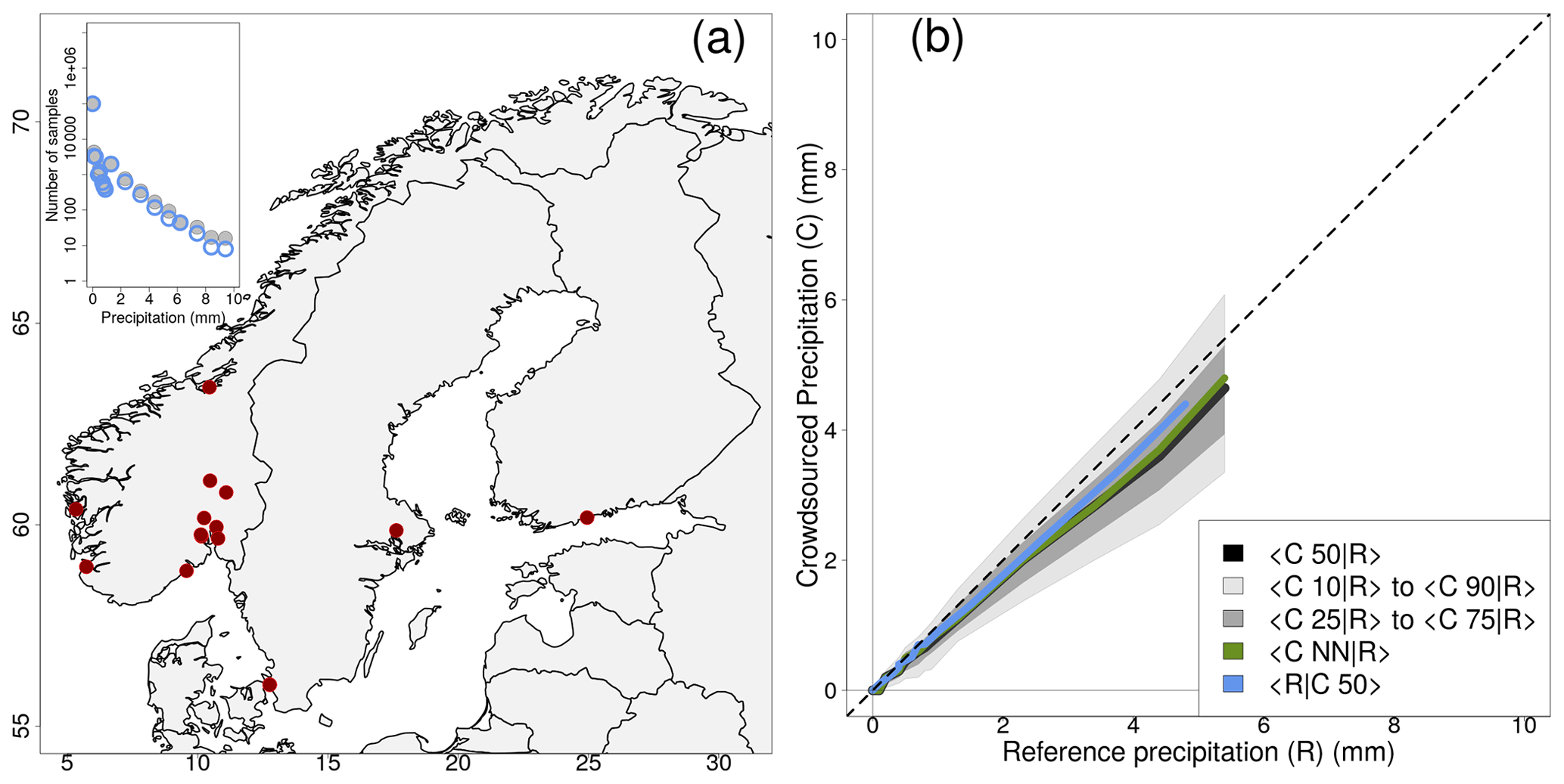
Figure 1 Empirical distribution of crowdsourced hourly precipitation totals (C) as a function of reference observations (R) based on measurements from 1 September 2019 to 1 November 2022. The crowdsourced stations used lie within circular regions of radius equal to 1 km from the reference stations and there must be at least 5 crowdsourced observations simultaneously available. Panel (a) shows the location of the 15 reference stations and the inset on the top right shows the number of observations as a function of the precipitation classes (see Sect. 3). Panel (b) shows aggregated statistics (i.e. median over all samples) on C conditional to R, such as: the crowdsourced observation nearest to the reference (green, NN in the legend stands for nearest neighbour); the median of all observations within the circular region (black); the IQR (i.e. interquartile range, dark gray shaded area); the IDR (i.e. interdecile range, light gray shaded area).

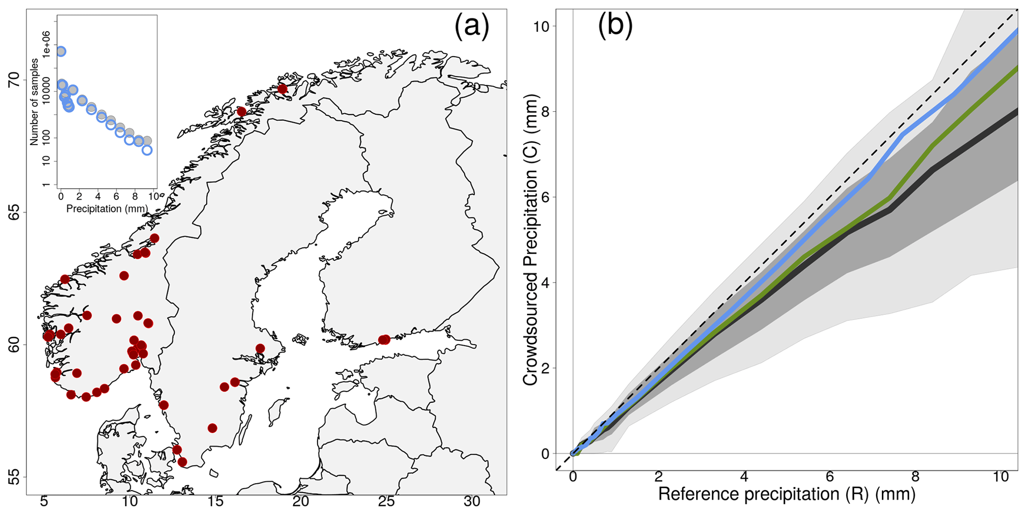
Figure 2 Empirical distribution of crowdsourced hourly precipitation totals (C) as a function of reference observations (R) based on measurements from 1 September 2019 to 1 November 2022. The crowdsourced stations used lie within a circular region of radius equal to 3 km from the reference stations. We have used only those cases when at least 10 crowdsourced observations were simultaneously available. Panel (a) shows the location of the 51 reference stations. The layout is similar to Fig. 1.

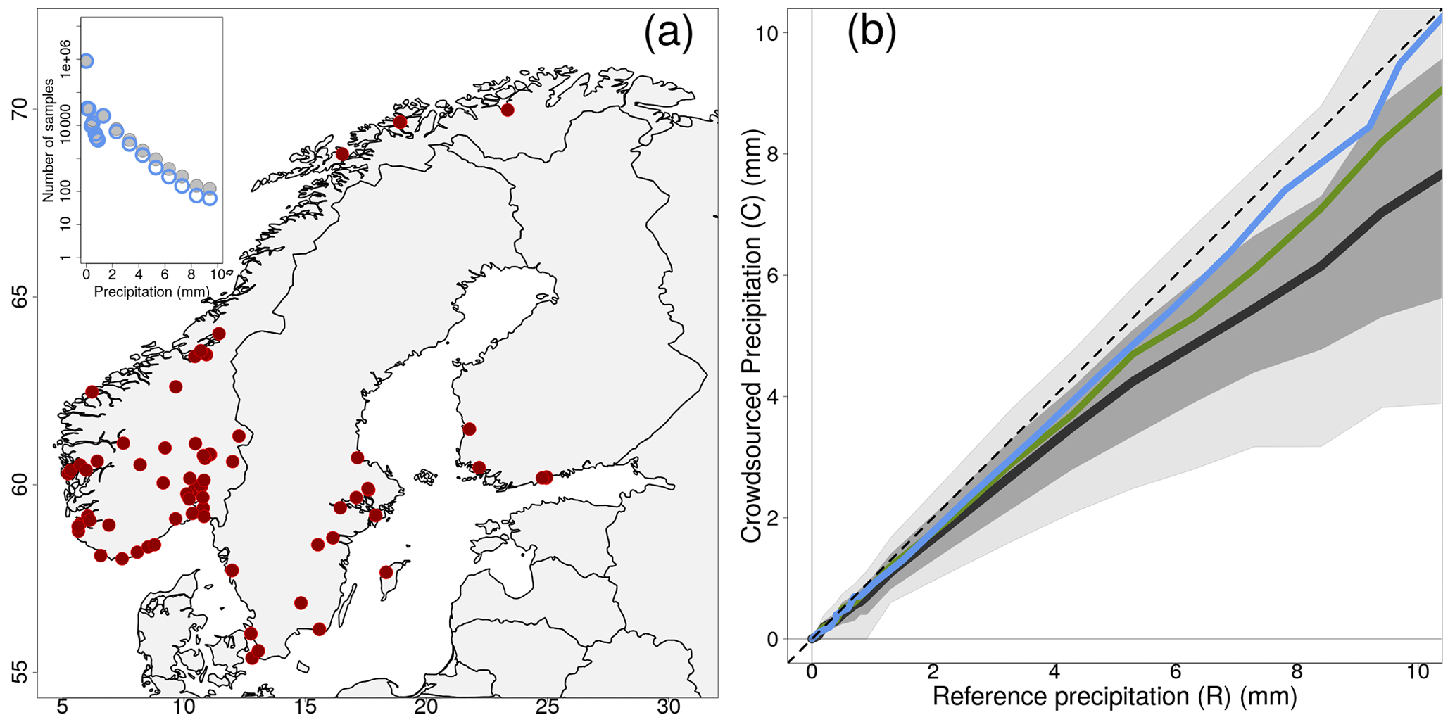
Figure 3 Empirical distribution of crowdsourced hourly precipitation totals (C) as a function of reference observations (R) based on measurements from 1 September 2019 to 1 November 2022. The crowdsourced stations used lie within circular regions of radius equal to 5 km from the reference stations. We have used only those cases when at least 10 crowdsourced observations were simultaneously available. Panel (a) shows the location of the 81 reference stations. The layout is similar to Fig. 1.

The procedure used to collect the samples for the study is the following. Given the reference stations in Figs. 1–3, we collect one “sample” for each station every hour. Each sample is a collection of the following values (or records): the reference observed value R; the observed value of the nearest crowdsourced rain gauge C_NN; percentiles from the distribution of the crowdsourced observations, such as: the 10th C₁₀, the 25th C₂₅, the median C₅₀, the 75th C₇₅ and the 90th C₉₀. We are considering percentiles because they provide more robust (i.e. less dependent on prior assumptions on probability distribution functions that precipitation should follow) and resistant (i.e. less influenced by outliers) estimates (Lanzante, 1996). Then, aggregated statistics of each record over all samples are calculated with several different mathematical operators, depending on the specific elaboration or score we want to compute. The aggregated statistics will be indicated with the symbol 〈 … 〉 (e.g. 〈R〉 indicates the aggregated statistics of the reference observed values over all samples).

Precipitation measurement uncertainties follow a multiplicative error model (Tian et al., 2013), as a consequence our assessment takes into account that observation uncertainty increases with the amount. This leads us to define a number of precipitation classes for hourly precipitation amounts, which we will use to stratify the input samples and, consequently, the outcomes of our study. The classes with respect to the generic record X (either one of R or C₅₀, as we will see in the following) are (units are mm): $\mathrm{0}\le X<\mathrm{0.1}$, $\mathrm{0.1}\le X<\mathrm{0.2}$, …, $\mathrm{0.9}\le X<\mathrm{1}$, 1≤X2, $\mathrm{2}\le X<\mathrm{3}$, …, $\mathrm{9}\le X<\mathrm{10}$. The whole list of classes is reported in the first column of Tables 1–3.

Table 1 Statistics of the empirical distribution of crowdsourced observations conditional to classes of reference precipitation R based on measurements from 1 September 2019 to 1 November 2022. The crowdsourced stations used lie within circular regions of radius equal to 1 km from the reference stations and there must be at least 5 crowdsourced observations simultaneously available. The data shown in the table have been used to obtain the graph in Fig. 1b. The first column reports the definitions of the precipitation classes. The second column is the number of samples in a class n, besides n^* shown in brackets is the number of samples when the classes are defined with respect to C₅₀ (e.g. … ≤C₅₀〉 …). For the symbols in the remaining three columns see Sect. 3. Note that in the column 〈C_NN|R〉, the relative difference between 〈C_NN|R〉 and 〈R〉 is reported in brackets (only when $|\langle C_{\mathrm{NN}}|R\rangle -\langle R\rangle |>\mathrm{0.1}$ mm). In the last column, the 5-tuple is the set of percentiles and the closest to 〈R〉 is shown in bold (more than one bold value is admissible for ties).

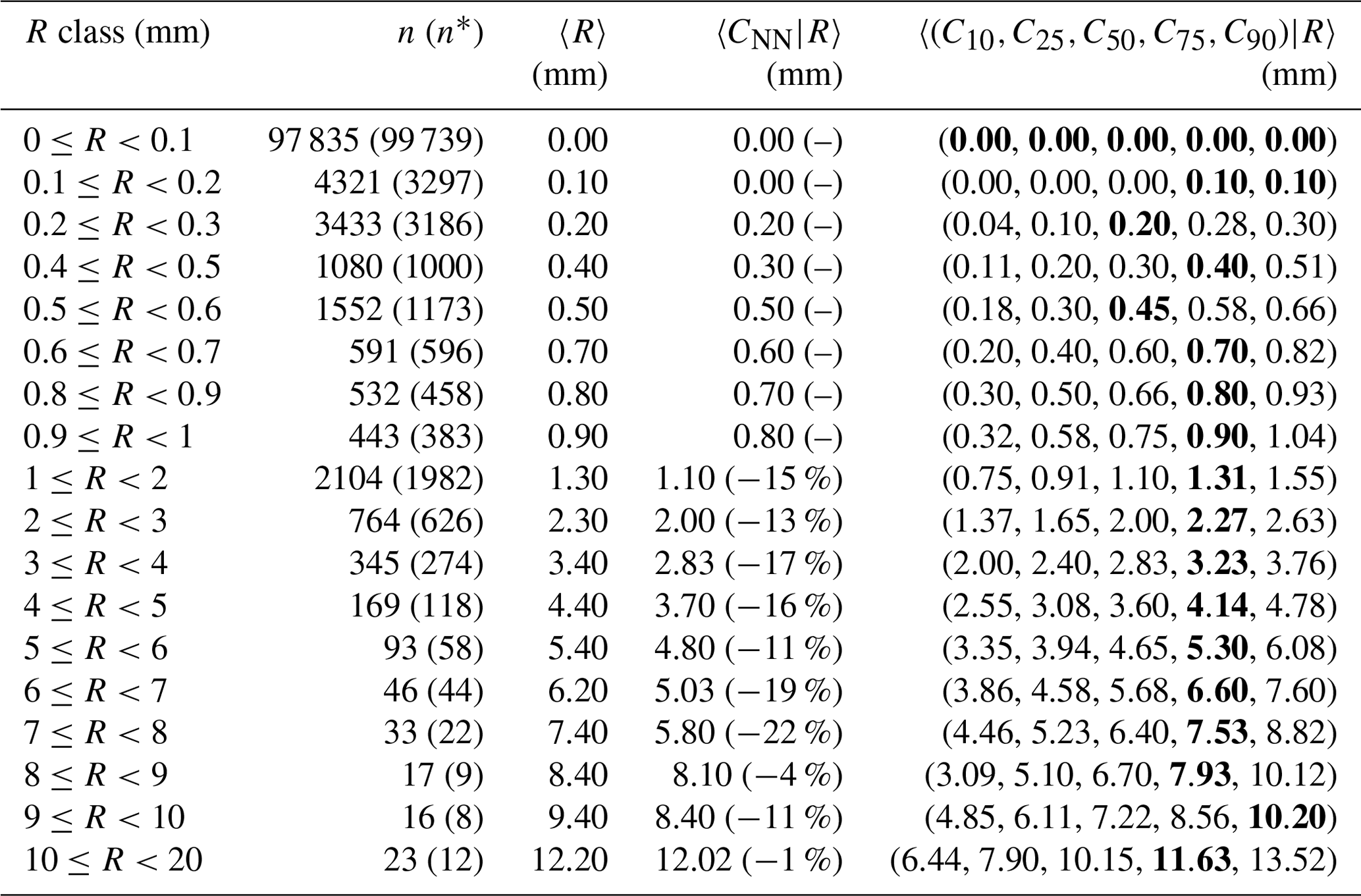
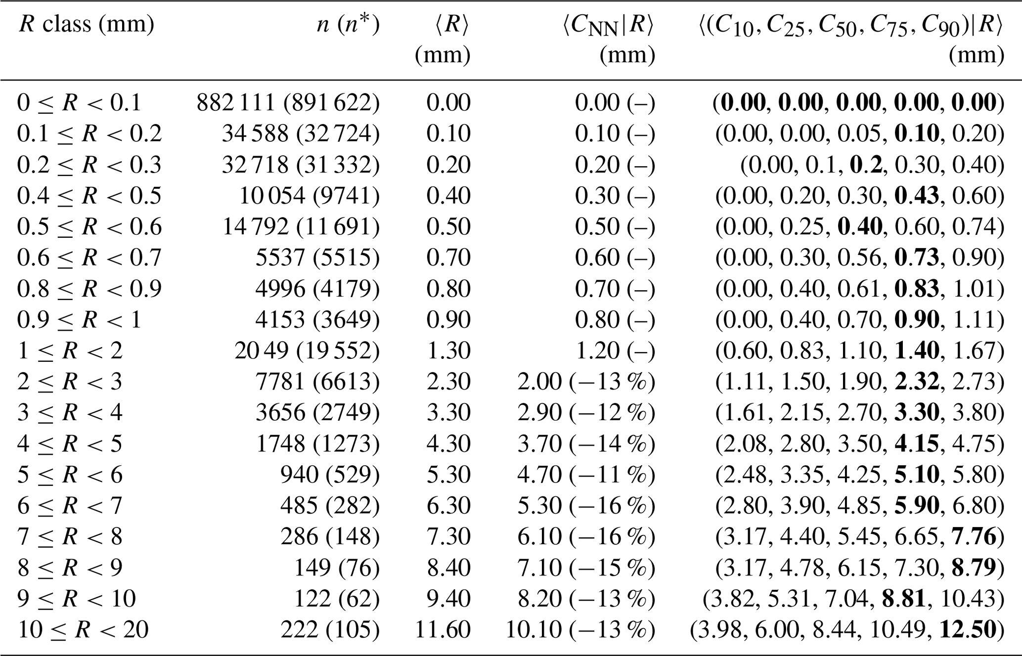
Table 2 Statistics of the empirical distribution of crowdsourced observations conditional to classes of reference precipitation R based on measurements from 1 September  019 to 1 November 2022. The crowdsourced stations used lie within circular regions of radius equal to 3 km from the reference stations and there must be at least 10 crowdsourced observations simultaneously available. The data shown in the table have been used to obtain the graph in Fig. 2b. The layout is similar to Table 1.

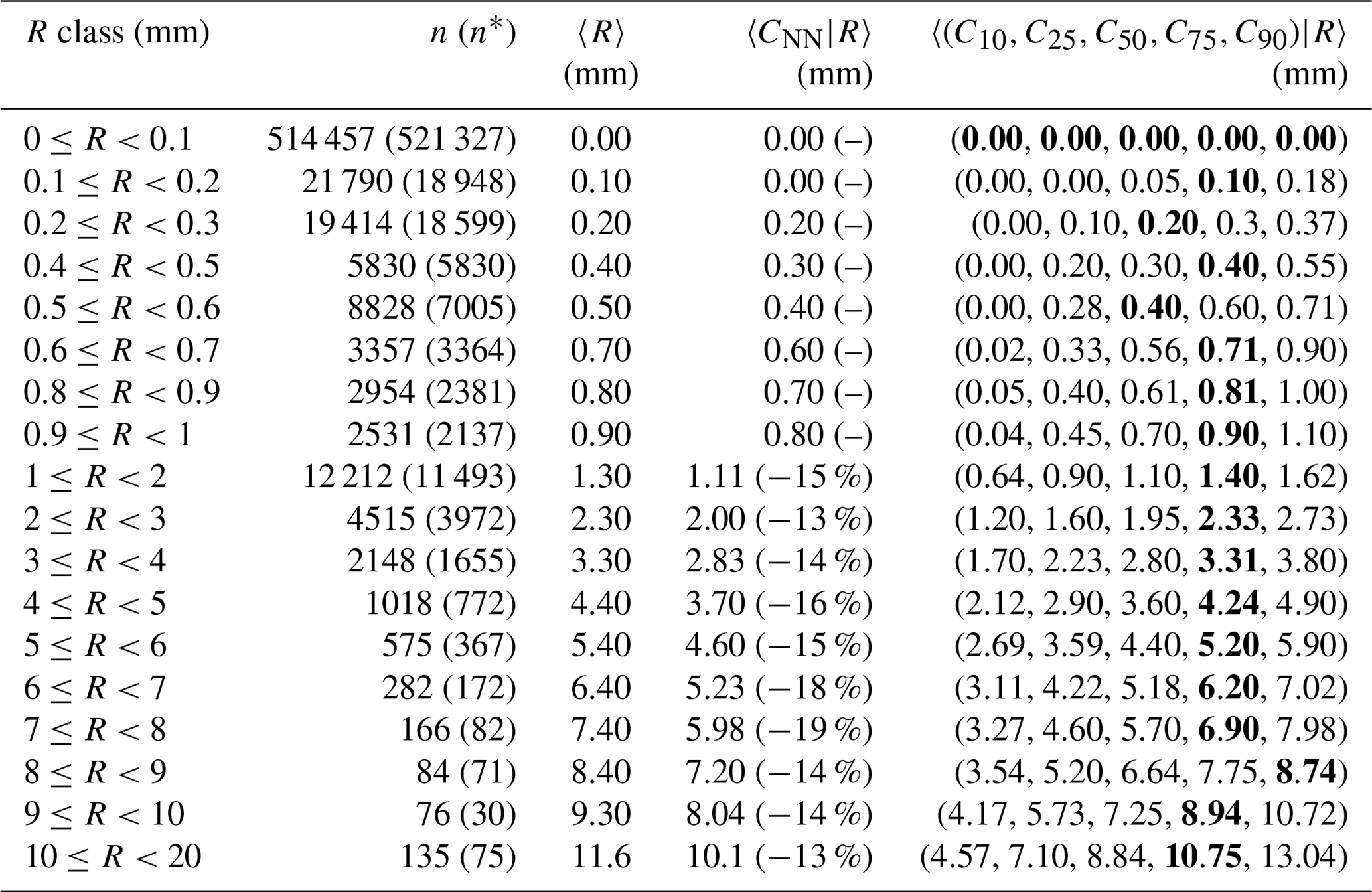
Table 3 Statistics of the empirical distribution of crowdsourced observations conditional to classes of reference precipitation R based on measurements from 1 September 2019 to 1 November 2022. The crowdsourced stations used lie within circular regions of radius equal to 5 km from the reference stations and there must be at least 10 crowdsourced observations simultaneously available. The data shown in the table have been used to obtain the graph in Fig. 3b. The layout is similar to Table 1.

Considering the climatology of hourly precipitation in Scandinavia, most of the samples should refer to situations of no- or light precipitation (from 0.1 to 2 mm). Then, the number of samples will decrease for increasing precipitation amounts. The exact number of samples in each class is reported in Tables 1–3 (second columns) and it is shown in the upper-right insets of Figs. 1a–3a (the y-axis has a logarithmic scale). Note that when R is used to distinguish between the classes (i.e. X=R in the definition of classes above), this corresponds to n in the tables and the gray dots in the figures. Alternatively, when X=C₅₀, this corresponds to n^* in the tables and blue dots in the figures. It is worth remarking that not all results reported in the tables are shown in the figures. In particular, in the figures, we show values between 0 and 10 mm and we require at least 60 samples (n>60) within a class in order to show the aggregated statistics. The choice is based on the fact that in the figures we do not want to compare with each other values characterized by rather different uncertainties. In the tables, the choice is left to the readers.

In Tables 1–3, for the class $\mathrm{0}\le X<\mathrm{0.1}$ (i.e. first row in the tables) n^* is always higher than n. Then, for classes where the maximum precipitation amount is below 1 mm, we still have some cases when n^* exceeds n. This never happens for classes referring to amounts higher than 1 mm and the deviations become greater as the amount increases. This mismatch between crowdsourced and reference precipitation in the frequency of occurrence of several classes, especially those with more intense precipitation, will be further investigated in Sect. 3.1.

3.1 Comparison of crowdsourced data against traditional observations

The distributions of crowdsourced precipitation conditional to (classes of) reference precipitation amounts have been computed and they are reported in Tables 1–3. Besides, in Figs. 1b–3b, the black lines and the gray shaded regions show an estimate of the distribution of crowdsourced precipitation conditional to reference precipitation amounts (i.e. R is now a continuous range of values, instead of a set of discretized classes). Figures show “estimates” obtained from the data in the tables, in the sense that we begin our elaboration by classifying our samples with respect to R. Then, for each of the classes, the aggregated statistics over all samples for every record is obtained using the median as the aggregation operator. This procedure is indicated with the following notation e.g. 〈C₅₀|R〉 that stands for: the median over all samples (i.e. 〈 … 〉; remember one sample corresponds to one hour) of the median of the crowdsourced observations (C₅₀) within a circular region surrounding a reference station, when we select only those samples belonging to a specific precipitation class (R). The aggregated statistics are then reported in Tables 1–3, in the third (〈C_NN|R〉) and fourth columns (the 5-tuple 〈C_x|R〉, with $x=\mathit{\{}\mathrm{10},\mathrm{25},\mathrm{50},\mathrm{75},\mathrm{90}\mathit{\}}$). In the second column, 〈R〉 is the median over all samples of all R values within a class. From the tables, we build the figures. Let us consider the thick black line in Fig. 1, which show 〈C₅₀|R〉 when r=1 km, the line is obtained by joining together the pairs of points (〈R〉, 〈C₅₀|R〉) in Table 1. Similar procedures apply for all the other lines and for the shaded regions. The light gray region spans the area between 〈C₁₀|R〉 and 〈C₉₀|R〉 (i.e. the interdecile range or IDR in brief). The dark gray region spans the area between 〈C₂₅|R〉 and 〈C₇₅|R〉 (i.e. the interquartile range or IQR). The two shaded areas give an indication of the variability expected on crowdsourced data given a reference precipitation amount; we will explore these aspects in more detail in Sect. 3.2. It is however worth noting that the IDR and the IQR are rather symmetric around 〈C₅₀|R〉. The graphs of Figs. 1b–3b show something more: the green line is 〈C_NN|R〉 and the blue line is 〈R|C₅₀〉. The latter is an aggregated statistics conditional to the crowdsourced precipitation amounts, which is defined as the median of R over all samples within a circular region surrounding a reference station, when we select only those samples with C₅₀ belonging to a specific precipitation class. Sometimes, the lines in Fig. 1 do not cover the whole range of reference precipitation values because for higher amounts we do not have enough samples (see Sect. 3).

The results in Tables 1–3 show that 〈R〉 is always included in the IDR of the crowdsourced observations and often it is within the IQR. However, we can notice a sort of drift in the positioning of 〈R〉 within the distributions. In the first lines, 〈R〉 stands close to the median 〈C₅₀|R〉, then it gradually moves towards the higher percentiles. For instance, 〈R〉 is in between 〈C₅₀|R〉 and 〈C₇₅|R〉 up until the classes: $\mathrm{8}\le R<\mathrm{9}$ (r=1 km); $\mathrm{7}\le R<\mathrm{8}$ (r=3 km); $\mathrm{6}\le R<\mathrm{7}$ (r=5 km). Then, for even higher amounts, 〈R〉 falls often between 〈C₇₅|R〉 and 〈C₉₀|R〉. The “drifting” of R within the crowdsourced distributions is also shown in Figs. 1–3 (i.e. the gradual increase in the deviation between the dashed and the thick black lines, as measured using the gray shaded areas as references). In the ideal situation of the reference and crowdsourced precipitation being random variables having the same probability density function, one should expect the line of 〈C₅₀|R〉 to lie on the identity line (the black dashed line) and the gray regions to be centered on that line too. This is not a bad assumption for classes of light precipitation (vast majority of the cases) but it becomes an increasingly less good approximation as the amount increases.

The blue lines in Figs. 1–3, on the other hand, show that 〈R|C₅₀〉 stay close to the identity line even for the highest precipitation classes. This means that we can rely on C₅₀ as an estimator of R across the range of precipitation amounts. However, for the higher values there is a systematic underestimation in the frequency of occurrence of those events, as pointed out in Sect. 3 when discussing on the differences between n and n^* in Tables 1–3.

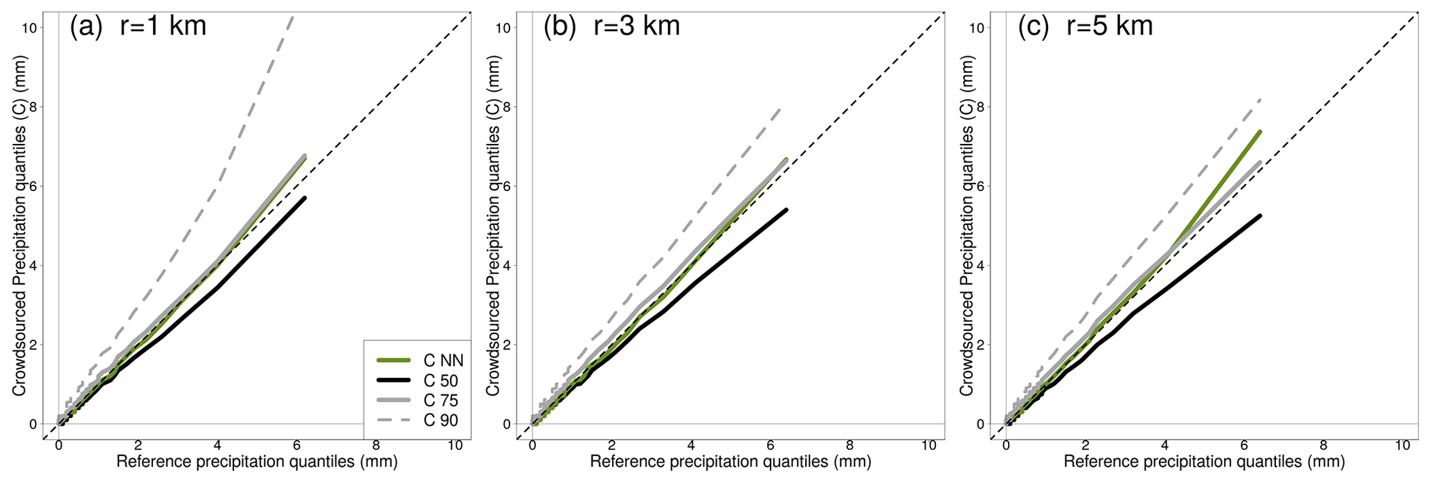
Figure 4 Quantile–quantile (Q–Q) plots comparing reference and crowdsourced hourly precipitation. The datasets are the same used for Figs. 1–3 and the three panels refer to the three neighbourhood sizes r=1, 3, 5 km. The crowdsourced variables are listed in the legend, with reference to Sect. 3 for the meaning of the symbols.

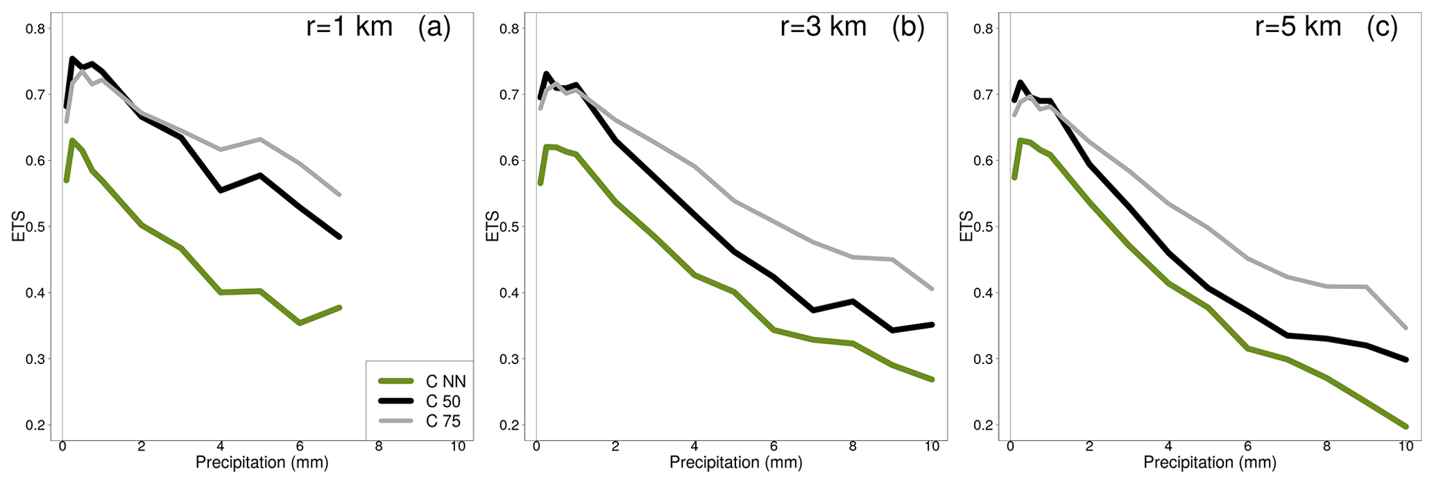
Figure 5 Equitable threat score (ETS) comparing reference and crowdsourced hourly precipitation. The datasets are the same used for Figs. 1–3 and the three panels refer to the three neighbourhood sizes reported (r equal to 1, 3 and 5 km). The green line shows the ETS for the crowdsourced observation nearest to the reference. The black and the gray lines show the ETS for selected percentiles of the crowdsourced observations within the neighbourhood.

Since the aggregated statistics in the last column of Tables 1–3 involve regionalization of point values into values representative of an area, then part of the underestimation may be due to the smoothing inherent in the regionalization processes (or “conditional bias”; Wilks, 2019). It is then interesting to consider 〈C_NN|R〉 (fourth column in the tables or the green lines in the figures), since in this case we are comparing point values against point values and we should not expect conditional biases. The tables shows that 〈R〉 and 〈C_NN|R〉 do have very similar values (between ±0.1mm) for precipitation classes below: 1 mm (r=1 and r=3 km); 2 mm (r=5 km). Then, 〈C_NN|R〉 underestimates 〈R〉 and the relative differences are within the range of values: −22 % and −1 % (r=1 km); −19 % and −13 % (r=3 km); −16 % and −11 % (r=5 km).

The empirical distributions of crowdsourced and reference hourly precipitation observations are compared in the quantile–quantile (Q–Q) plots shown in Fig. 4. The thin-dashed black lines mark the identity lines y=x, which is where the points would lie if the two distributions were similar. We point out that: (i) the Q–Q plots for both C₇₅ and C_NN stays close enough to the identity line; (ii) the graphs in the three panels are rather similar among each other, although a slight worsening of the agreement can be noticed as the distance increases. It is worth remarking that the crowdsourced data have not been quality controlled, then the higher quantiles are most likely affected by outliers (e.g. C₉₀ in Fig. 4a). Looking at the figure, it is possible to state that a Q–Q mapping procedure (Wilks, 2019) might be a good way to deal with some of the underestimation issues we have reported above.

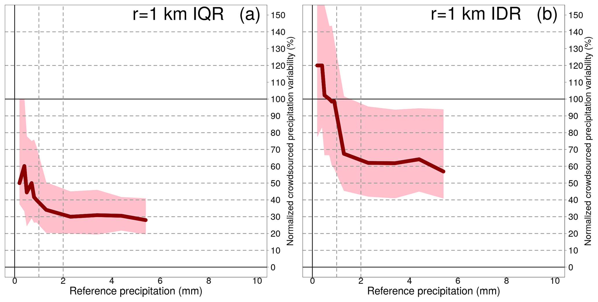
Figure 6 Spatial variability of crowdsourced hourly precipitation as a function of reference precipitation amounts, within circular regions of 1 km radius. IQR stands for interquartile range, while IDR stands for interdecile range. The dataset used, the reference precipitation classes and the constraints imposed are the same as for Fig. 1. In panel (a), The tick red lines show the median of the IQRs (IDRs in panel b) within the precipitation classes. In panel a, The shaded pink regions delimit the area between the 25th and the 75th percentiles of the IQRs (IDRs in panel b).

Figure 7 Spatial variability of crowdsourced hourly precipitation as a function of reference precipitation amounts, within circular regions of 3 km radius. The layout is similar to Fig. 6 and the dataset used is the same as that used in Fig. 2.

The last result we present in this section focuses on the performances of crowdsourced observations in distinguishing between precipitation yes/no cases and, more in general, on the agreement between crowdsourced and reference precipitation being simultaneously above predefined thresholds. In Fig. 5, the equitable threat score (ETS, Jolliffe and Stephenson, 2012) of the crowdsourced precipitation is shown for the three neighbourhoods used in our study. Given a threshold of precipitation (on the x-axis), the ETS measures the fraction of crowdsourced observations that were correctly predicting an amount above that threshold, adjusted for the hits associated with random chance. A “hit” is defined as “both the crowdsourced observation (or derived statistics) and the reference are greater than the threshold”. Because of the differences between n and n^* (see Sect. 3), we should expect an increase of “misses” when the amount increases (i.e. “the crowdsourced observation is below the threshold, while the reference is above”). The ETS graphs show that we can have good confidence in the ability of crowdsourced data in distinguishing between precipitation yes/no events. As expected, performance deteriorates with increasing precipitation. The aggregation of crowdsourced data over small regions yields somewhat better and more stable results, as can be seen in the graphs by comparing the results for the nearest neighbours (green line) and those for the aggregated statistics (black and – especially – the gray line).

3.2 Spatial variability of precipitation

The spatial variability of precipitation over neighbourhoods of 1, 3 and 5 km has been measured using the IDR (i.e. $\langle (C_{\mathrm{90}}-C_{\mathrm{10}})|R\rangle$) and the IQR (i.e. $\langle (C_{\mathrm{75}}-C_{\mathrm{25}})|R\rangle$). Given a neighbourhood, IDR gives an idea of the total range of values we should expect to find in the crowdsourced observations, extreme values included. IQR represents the typical (i.e. most likely) range of values. Variability is assumed to depend on precipitation intensity, then we will present our results using the same precipitation classes defined in Sect. 3.

Figure 8 Spatial variability of crowdsourced hourly precipitation as a function of reference precipitation amounts, within circular regions of 5 km radius. The layout is similar to Fig. 6 and the dataset used is the same as that used in Fig. 3.

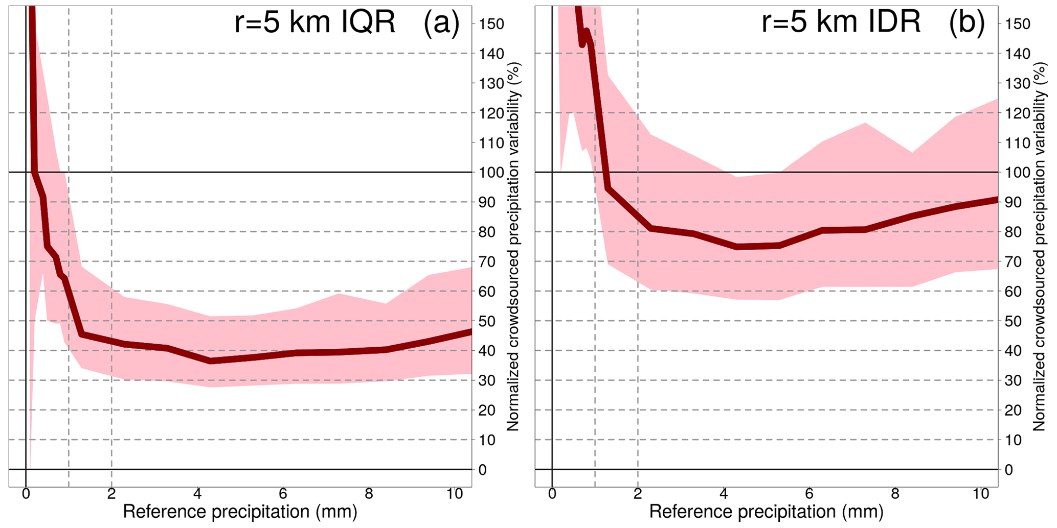
Table 4 Spatial variability of crowdsourced observations conditional to classes of reference precipitation R based on measurements from 1 September 2019 to 1 November 2022. The crowdsourced stations used lie within circular regions of radius equal to 1 km from the reference stations and there must be at least 5 crowdsourced observations simultaneously available. The data shown in the table have been used to obtain the graph in Fig. 6. The first column reports the definitions of precipitation classes. For the notation in the remaining three columns, see Sect. 3. The second (fourth) column is equivalent to $\langle C_{\mathrm{90}}-C_{\mathrm{10}}|R\rangle$ ($\langle C_{\mathrm{75}}-C_{\mathrm{25}}|R\rangle$). The 3-tuple in these columns show the results with three different aggregation operators 〈 … 〉, which are over all samples in each class: (25th percentile, median (bold), 75th percentile). The third (fifth) column is the normalized IDR (IQR), which is defined as $\langle C_{\mathrm{90}}-C_{\mathrm{10}}|R\rangle /\langle C_{\mathrm{50}}|R\rangle$ ($\langle C_{\mathrm{75}}-C_{\mathrm{25}}|R\rangle /\langle C_{\mathrm{50}}|R\rangle$). The 3-tuple in these columns show the results with three different aggregation operators, as for the second and fourth columns, with the difference that the operator used for 〈C₅₀|R〉 is always the median (i.e. 〈C₅₀|R〉 is constant over each 3-tuple).

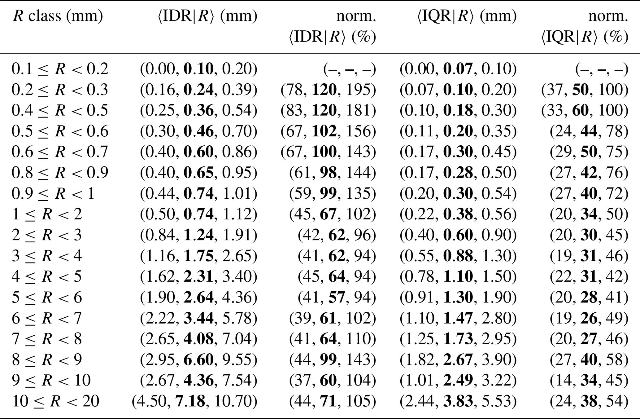
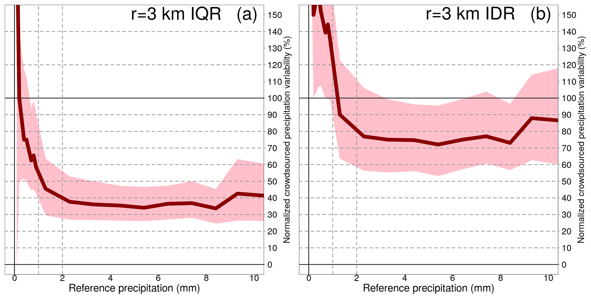
Table 5 Spatial variability of crowdsourced observations conditional to classes of reference precipitation R based on measurements from 1 September 2019 to 1 November 2022. The crowdsourced stations used lie within circular regions of radius equal to 3 km from the reference stations and there must be at least 10 crowdsourced observations simultaneously available. The data shown in the table have been used to obtain the graph in Fig. 7. The table layout is similar to Table 4.

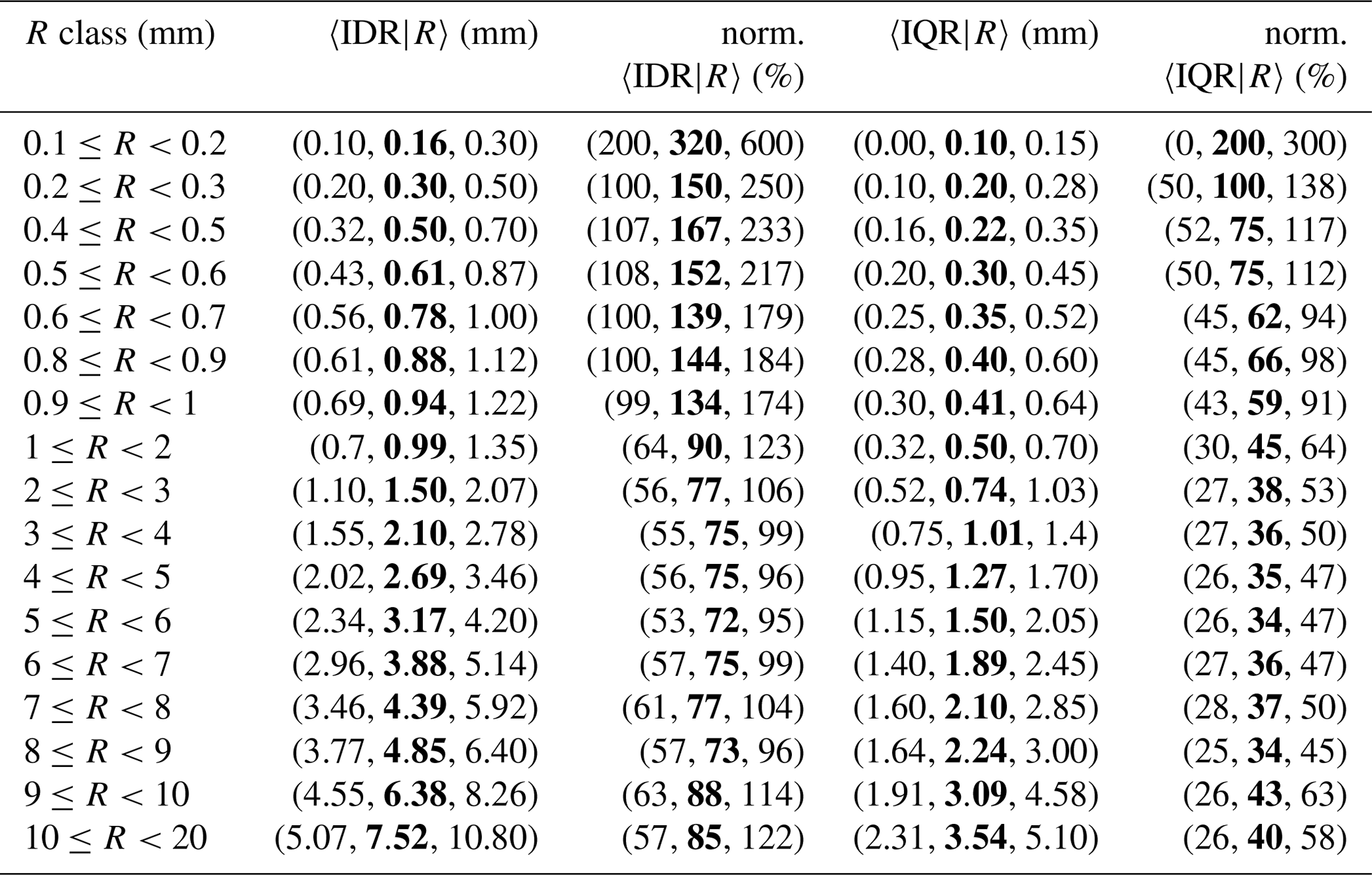
Table 6 Spatial variability of crowdsourced observations conditional to classes of reference precipitation R based on measurements from 1 September 2019 to 1 November 2022. The crowdsourced stations used lie within circular regions of radius equal to 5 km from the reference stations and there must be at least 10 crowdsourced observations simultaneously available. The data shown in the table have been used to obtain the graph in Fig. 8. The table layout is similar to Table 4.

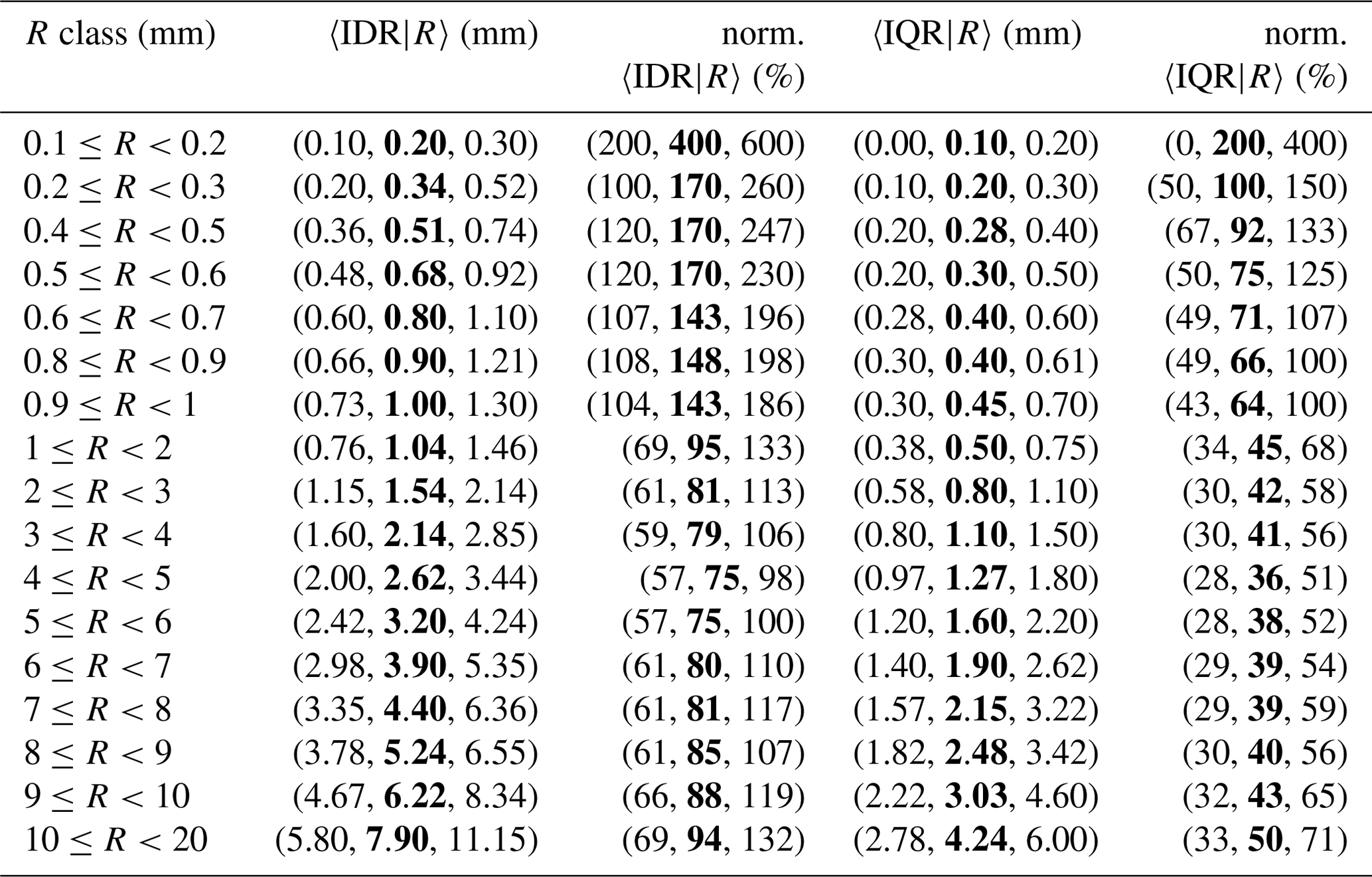
The results are presented in Tables 4–6 and Figs. 6–8 for the three neighbourhoods. In both figures and tables, we have used the normalized crowdsourced variability (units %), where the normalization of the spread is meant with respect to the observed amount. We have used three different aggregation operators 〈 … 〉, which are: the 25th, the 50th (median) and the 75th percentiles of all samples within a class. Then, for instance, in Table 4, the 3-tuple in the first row of the second column (〈IDR|R〉, units mm) is (0.00, 0.10, 0.20) and it means: 0.00 mm is the 25th percentile of all IDR samples within the class $\mathrm{0.1}\le R<\mathrm{0.2}$; 0.10 mm is the median of all IDR samples within the same class; 0.20 mm is the 75th percentile of all IDR samples within the same class. Since we are using the spread of the crowdsourced observation, the normalization is done on the basis of 〈C₅₀|R〉 (and not of 〈R〉). Then, the normalized IDR (IQR) is defined as $\langle C_{\mathrm{90}}-C_{\mathrm{10}}|R\rangle /\langle C_{\mathrm{50}}|R\rangle$ ($\langle C_{\mathrm{75}}-C_{\mathrm{25}}|R\rangle /\langle C_{\mathrm{50}}|R\rangle$). Note that, for the results presented in this section, the operator used in the aggregation of 〈C₅₀|〉 is always the median over the samples (i.e. even when calculating the 25th percentile of e.g. $\langle C_{\mathrm{90}}-C_{\mathrm{10}}|R\rangle /\langle C_{\mathrm{50}}|R\rangle$, we have used the median to obtain 〈C₅₀|R〉). In the tables, the absolute values of the variability are reported (i.e. $\langle \mathrm{IDR}|R\rangle \equiv \langle C_{\mathrm{90}}-C_{\mathrm{10}}|R\rangle$ and $\langle \mathrm{IQR}|R\rangle \equiv \langle C_{\mathrm{75}}-C_{\mathrm{25}}|R\rangle$) but not on the figures.

The link between figures and tables is explained with an example. Let us consider Fig. 7a, the pink area shows the range of values delimited by the first and the third values of the 3-tuple in the fifth column of Table 5 (i.e. the range of values for the normalized 〈IQR|R〉, between the 25th and the 75th percentiles). The thick red line joins together the second values of the 3-tuple in the fifth column of Table 5 (i.e. the medians of norm. 〈IQR|R〉). Then, the pink area is the variability we have found in the normalized crowdsourced variability. The thick red line is the “typical” value of the normalized crowdsourced variability.

A common feature of all the three figures is that the normalized spatial variability is very high for light precipitation (i.e. less than 1 mm), often even with values higher than 100 %. Then, the normalized variability stabilizes and reaches a plateau which remains fairly constant throughout the range of precipitation amounts. As expected, the variability increases as the area of the neighbourhood considered increases too.

For the IQRs, the plateaus, reached for values ≥2 mm, are (we consider the medians here): between 26 % and 40 % (1 km); between 34 % and 43 % (3 km); between 36 % and 50 % (5 km). For the IDRs, the plateaus, reached for values higher than 2 mm, are: between 57 % and 99 % (1 km); between 72 % and 88 % (3 km); between 75 % and 94 % (5 km).

4 Conclusions

The relationship between the empirical distributions of Netatmo's hourly precipitation totals conditional to reference precipitation has been investigated. We have found that the reference observations are always included in the envelope of the empirical distribution of crowdsourced data (i.e. between the 10th and the 90th percentiles). However, there are indications that for intense precipitation crowdsourced data may underestimate precipitation. This is inline with WMO guidelines, which recommend to correct measurements from tipping-buckets rain gauges and to adjust measurements of different rain gauges to make them more comparable.

The results obtained by comparing the empirical distributions of crowdsourced and reference precipitation suggest that it would probably be possible to use a quantile-quantile mapping procedure to adjust the crowdsourced observations toward the reference values.

It might also be beneficial to aggregate the crowdsourced data over small neighbourhoods, of the size of 1 to 5 km, instead of using the raw data. In this way, crowdsourced data performs better in distinguishing between precipitation yes/no events, for instance.

The investigation of the crowdsourced precipitation spatial variability shows that when comparing measurement from two points, even if not very far from each other (i.e. distance between 1 to 5 km), one should not be surprised to find values that are quite different from each other (up to 50 % of the mean hourly precipitation in the area). The variability is quantified in detail in the presented tables. The results are representative of the actual spatial variability of precipitation over small distances, as described in Sect. 3. However, part of the variability is certainly given by the not ideal siting exposure of Netatmo's stations and, in this sense, the results obtained can be considered as a maximum estimate of the variability.