Response of the atmospheric boundary layer to SST variability in a coupled simulation in the Atlantic trades

The coupling between the atmosphere and the ocean at the oceanic mesoscale (∼100–1000 km) plays a significant role in shaping the energy exchanges between the two fluids. We investigate how such coupling is represented in a state-of-the-art high resolution ocean-atmosphere coupled numerical simulation. In particular, we look into the thermodynamic adjustment of the marine atmospheric boundary layer (MABL) to sea surface temperature (SST) spatial anomalies. Mesoscale SST impacts the lower-tropospheric static stability by modifying the surface turbulent fluxes; these changes can be traced up to the top of MABL as a consequence of the modified air column buoyancy, with a subsequent impact on MABL top entrainment fluxes. Alongside, MABL temperature is found to partially adjust to SST, whereas MABL humidity does not, as surface evaporation and the entrainment of dry air mass at top-of-MABL have opposing effects which partially balance out: this results in a high sensitivity (∼25 % K⁻¹) of the anomalous surface latent heat fluxes to mesoscale SST anomalies. Our findings, thus, indicate that small scale SST variability can have upscaling effects on the surface energy exchanges via non-linear MABL responses.

1 Introduction

With the ongoing rise in global temperatures, the larger moisture input from the oceans into the atmosphere is expected to be due to enhanced surface fluxes, that are tightly related to the lower atmospheric mixing and low-level cloud feedbacks (e.g. Vogel et al., 2022). Mesoscale (100–1000 km) and sub-mesoscale (10–100 km) sea surface temperature (SST) spatial structures, in particular, are of special importance in shaping air-sea interactions (Seo et al., 2023): understanding how dynamical and thermodynamic processes in the lower atmosphere and the upper ocean affect energy and mass exchanges between the two fluids is a compelling task in order to ameliorate climate projections (e.g. Sherwood et al., 2014). In particular, tropical oceans host shallow cumuli which are responsible for a significant fraction of future climate uncertainties (Bony and Dufresne, 2005; Bony et al., 2015): their presence is clearly affected by air-sea fluxes and at the same time can modify them.

The recent EUREC⁴A-ATOMIC field campaign (ElUcidating the RolE of Cloud–Circulation Coupling in ClimAte - Atlantic Tradewind Ocean–Atmosphere Mesoscale Interaction Campaign) (Stevens et al., 2021) provided a wealth of in-situ data including insightful information on how air and sea interact in the north-western tropical Atlantic. In this region, despite being characterized by relatively weak SST gradients, there is growing evidence that SST spatial variability can affect the marine atmospheric boundary layer (MABL) with implications for surface fluxes (Fernández et al., 2023; Borgnino et al., 2025) and low-level clouds (Acquistapace et al., 2022; Chen et al., 2023). In particular, Borgnino et al. (2025) have shown that the fact that MABL-top entrainment is enhanced over warm SST areas is responsible for a fast export of humidity in the free troposphere, which, in turn, keeps the surface latent heat flux high. As they used an atmospheric model forced by daily satellite-derived SST fields, goal of the present work is to test whether the MABL response to the SST variability highlighted in Borgnino et al. (2025) is found in a realistic high-resolution coupled ocean-atmosphere numerical simulation. This study addresses whether the inclusion of a fully three-dimensional ocean dynamics can significantly affect the MABL response to SST spatial variability and its impact on the surface turbulent heat fluxes. In Sect. 2 we present the coupled numerical model and the methods used, Sect. 3 discusses the main results and in Sect. 4 conclusions are summarized.

2 Data and methods

We analyze daily-averaged atmospheric fields from a coupled simulation performed with the Coastal and Regional Ocean Community (CROCO) model (Auclair et al., 2022) at 1 km grid spacing for the ocean and the Weather Research and Forecasting (WRF) model version 4.2.1 (Skamarock et al., 2019) at 2 km grid spacing for the atmosphere. The WRF configuration has 40 vertical eta levels, 15 of which in the lower 2 km of the atmosphere. The coupling is performed with the OASIS3-MCT coupler (Valcke et al., 2013) every hour and includes momentum, freshwater and turbulent heat fluxes. The model covers a 10° by 10° domain, specifically from (5° N, 62° W) to (15° N, 52° W) and the entire month of February 2020 is taken in consideration. More details on the model configuration, including the choice of the numerical parameterizations, can be found in Conejero et al. (2024), that investigate the relevance of the coupling between SST, ocean currents and surface wind at the meso- and sub-mesoscales.

All fields of interest are low-pass filtered with a Gaussian kernel with a standard deviation of 150 km, to be consistent with Borgnino et al. (2025), and the small-scale spatial anomaly is obtained by subtracting the smooth field from the original one according to

$$\begin{array}{}\text{(1)}& {\mathit{\psi }}^{\prime }=\mathit{\psi }-\stackrel{\mathrm{‾}}{\mathit{\psi }},\end{array}$$

where ψ is the original field, $\stackrel{\mathrm{‾}}{\mathit{\psi }}$ denotes the low-pass filtered field and ψ^′ the small-scale anomaly. We consider data at least 50 km far from the coastlines and from the lateral boundaries of the model in order to exclude circulation features arising either from coastal interactions and flow distortions at the model boundaries. Most of the fields analyzed are directly retrieved as model outputs. Daily averaged anomalies of SST, MABL height (MABLH), 2 m water vapor mixing ratio (q_2 m) and 2 m air temperature (T_2 m) visually suggest the different degree of coupling that atmospheric properties have with the SST (Fig. 1). As an overview, it is possible to say that SST structures imprint themselves on T_2 m and MABLH to a larger extent: anomalies of the same sign are vastly co-located in the provided snapshots. The emergence of atmospheric circulations aligned with the mean wind direction adds some noise to the signal we aim at investigating (as, for example, for MABLH and q_2 m). The same degree of accord with SST is not found for q_2 m, which seems to be less correlated to the surface thermal forcing, except in a few locations such as over an oceanic eddy at about 11° N, 59° W.

To estimate and discuss the scaling of the turbulent surface fluxes as a function of SST^′, we exploit their standard bulk formulations, namely

$$\begin{array}{}\text{(2)}& \begin{array}{rl}& \mathrm{SHF}={\mathit{\rho }}_{\mathrm{a}}{c}_p{C}_{\mathrm{h}}\left|{\mathit{u}}_{\mathrm{10}\mathrm{m}}\right|(\mathrm{SST}-T_{\mathrm{2}\mathrm{m}});\\ & \mathrm{LHF}={\mathit{\rho }}_{\mathrm{a}}{L}_{\mathrm{v}}{C}_{\mathrm{e}}\left|{\mathit{u}}_{\mathrm{10}\mathrm{m}}\right|\left(q^{*}\right(\mathrm{SST})-q_{\mathrm{2}\mathrm{m}}).\end{array}\end{array}$$

Turbulent fluxes are dependent on the wind speed close to the surface ($\left|{\mathit{u}}_{\mathrm{10}\mathrm{m}}\right|$) and are modulated by turbulent transfer coefficients (C_h and C_e) which, in general, have a weak dependence on environmental conditions (e.g. pressure and stability). Here we are interested in providing scaling laws for the main thermodynamic variables, hence air density is kept constant to a value of ${\mathit{\rho }}_{\mathrm{a}}=\mathrm{1.2}\mathrm{kg}{\mathrm{m}}^{-\mathrm{3}}$ given its negligible relative change at the sea surface; the turbulent transfer coefficients are set to values consistent with the conditions under investigation, $C_{\mathrm{h}}=C_{\mathrm{e}}=\mathrm{1.2}\times {\mathrm{10}}^{-\mathrm{3}}$ (Neggers et al., 2006). SHF, then, specifically depends on the temperature difference between the sea surface (SST) and the overlying air (T_2 m); whereas LHF takes into account the difference in saturation mixing ratio at sea surface q^*(SST), which follows the Clausius-Clapeyron law, and the atmospheric mixing ratio counterpart (q_2 m) (e.g. Fairall et al., 2003; Yu, 2009). Lastly, the specific heat at constant pressure $c_p=\mathrm{1004}\mathrm{J}{\mathrm{kg}}^{-\mathrm{1}}{\mathrm{K}}^{-\mathrm{1}}$ and the latent heat of vaporization $L_{\mathrm{v}}=\mathrm{2.5}\times {\mathrm{10}}^{\mathrm{6}}\mathrm{J}{\mathrm{kg}}^{-\mathrm{1}}$ are included for dimensional consistency.

From turbulent fluxes we can also compute the surface buoyancy flux (BF) following de Szoeke et al. (2021), as

$$\begin{array}{}\text{(3)}& \begin{array}{rl}\mathrm{BF}& ={\displaystyle \frac{g}{T_{\mathrm{v}}}}\stackrel{\mathrm{‾}}{w^{\prime }{T}_{\mathrm{v}}^{\prime }}={\displaystyle \frac{g}{T_{\mathrm{v}}}}\left(\stackrel{\mathrm{‾}}{w^{\prime }{T}^{\prime }}(\mathrm{1}+\mathit{\beta }q)+\stackrel{\mathrm{‾}}{w^{\prime }{q}^{\prime }}\mathit{\beta }T\right)\\ & =\underset{{\mathrm{SH}}_{\mathrm{term}}}{\underbrace{{\displaystyle \frac{g}{{\mathit{\rho }}_{\mathrm{a}}{T}_{\mathrm{v}}}}{\displaystyle \frac{\text{SHF}}{c_p}}(\mathrm{1}+\mathit{\beta }q)}}+\underset{{\mathrm{LH}}_{\mathrm{term}}}{\underbrace{{\displaystyle \frac{g}{{\mathit{\rho }}_{\mathrm{a}}{T}_{\mathrm{v}}}}{\displaystyle \frac{\text{LHF}}{L_{\mathrm{v}}}}\mathit{\beta }T}}\end{array}\end{array}$$

where $\stackrel{\mathrm{‾}}{w^{\prime }{T}_{\mathrm{v}}^{\prime }}$, $\stackrel{\mathrm{‾}}{w^{\prime }{T}^{\prime }}$ and $\stackrel{\mathrm{‾}}{w^{\prime }{q}^{\prime }}$ represent turbulent fluxes of virtual temperature, temperature (hence sensible heat flux, SHF) and moisture (i.e. evaporation, LHF); β is the ratio between the molar mass of moist air and that of dry air and it was set to 0.608 . We integrate the discussion by showing how the BF depends on the sensible heat flux terms (SH_term), latent heat flux terms (LH_term): we will be concerned both with the sensitivity of absolute magnitudes to SST and that between the corresponding mesoscale anomalies.

The Brunt-Väisäla frequency, indicative of the atmospheric dry static stability is computed as

$$\begin{array}{}\text{(4)}& N^{\mathrm{2}}={\displaystyle \frac{g}{\mathit{\theta }}}\cdot {\displaystyle \frac{\partial \mathit{\theta }}{\partial Z}},\end{array}$$

with g being the acceleration due to gravity, θ the potential air temperature and Z the geopotential height.

Vertical cross-sections of the atmospheric anomalies are drawn as a function of the surface SST anomaly to investigate the mean response of the MABL to the underlying SST forcing (see Fig. 3). On the vertical, pressure levels of the WRF model between the surface and 800 hPa are considered. On the horizontal, for a given pressure level, each SST^′ bin contains 5 % of the valid data considering all the grid points of the study area (as shown in Fig. 1) over the entire month of February 2020. Thus, for each level, we consider 20 bins of SST^′ with an equal number of values. In each bin we compute the mean, the standard deviation and the standard error of the mean of the corresponding atmospheric field anomaly, based on their spatial and temporal co-location with the SST^′ value. The statistical significance of the signals depends on the number of degrees of freedom which corresponds to the number of independent data. To estimate it, we first compute the autocorrelation in time for the spatial anomalies of the atmospheric field of interest, ψ^′. As this is about 1 d, we can consider daily fields to be independent from one another. Then, we compute their spatial autocorrelation lengths L_a∼30 km and we estimate the effective number of degrees of freedom as $N_{\mathrm{eff}}=\mathrm{\Omega }/L_{\mathrm{a}}^{\mathrm{2}}$, where Ω is the area in km² of the valid data, following Bretherton et al. (1999) and Meroni et al. (2018). This number of effective degrees of freedom is used, in each bin, to perform a two-tailed t test and detect signals that are significantly different from zero at the 95 % confidence level.

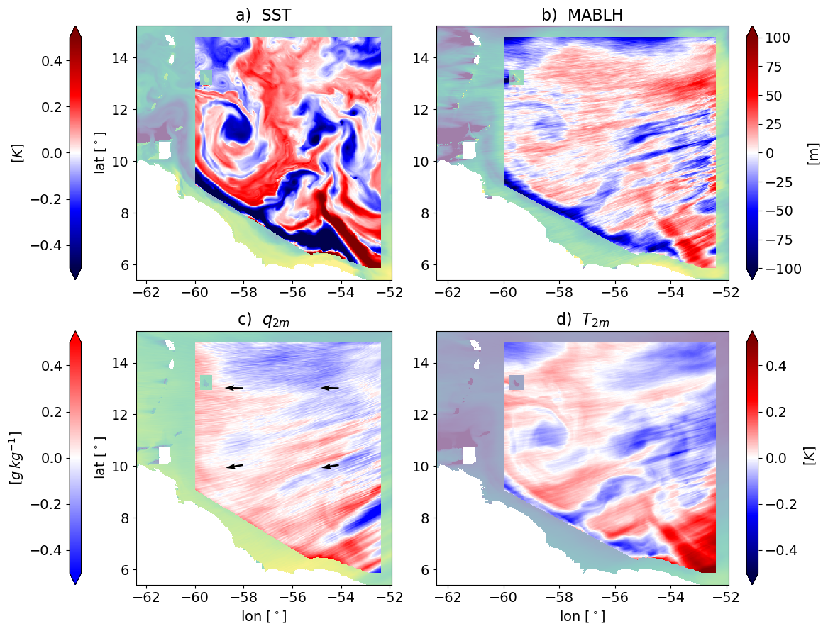
Figure 1 Daily averaged spatial anomalies of SST (a), MABL height (MABLH) (b), 2 m water vapor mixing ratio q_2 m (c) and 2 m air temperature T_2 m (d), on 1 February 2020. White and semi-transparent areas represent land and ocean zones that are neglected in the analyses. Arrows in panel (c) show the time-mean wind direction within the domain on the same day.

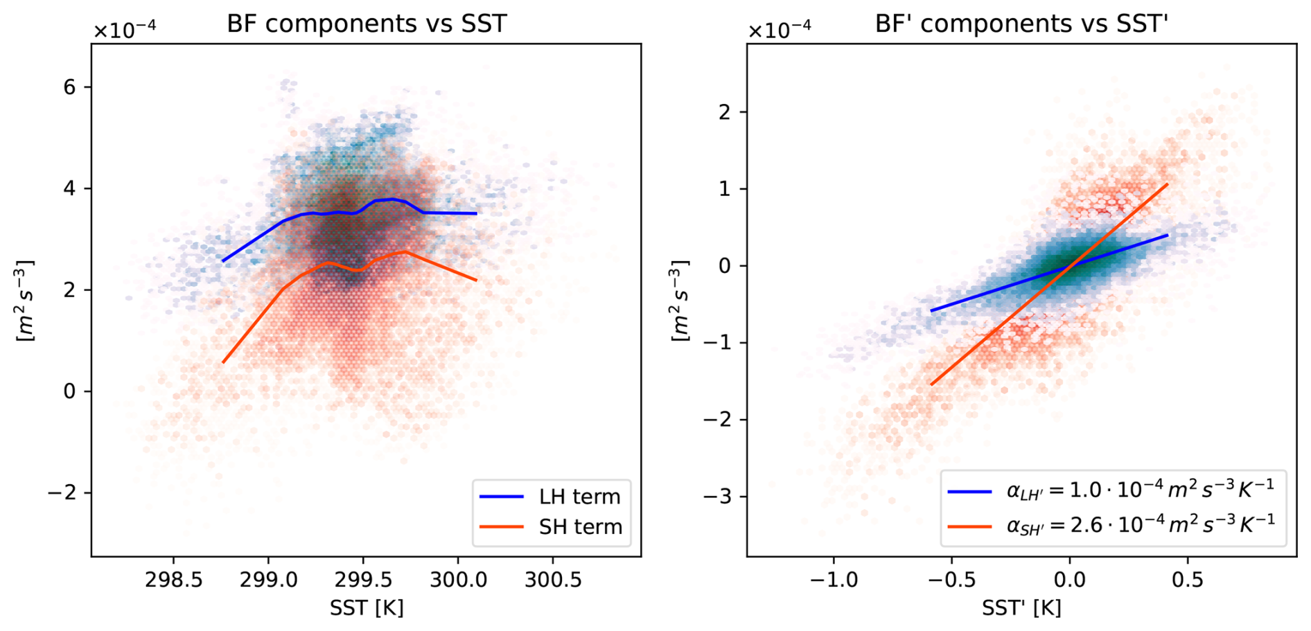
Figure 2 Analysis of magnitudes and sensitivity of the latent (LH, blue colours) and sensible (SH, orange colours) heat flux contributions to the total buoyancy flux (BF). We consider the unfiltered fields (left panel) and the corresponding mesoscale anomalies (right panel, filter sigma fixed at 150 km). The α coefficients in the legend of the right panel are the slopes ensuing from the linear regression drawn between mesoscale heat fluxes and SST^′.

3 Thermodynamic response

Enhanced evaporation and sensible heat exchange over warm SST anomalies lead to an increase of near surface air buoyancy, which is then redistributed within the air column through convection and turbulence up to MABL top. While at large scale air buoyancy production is generally dominated by evaporation (see Fig. 2, left panel), the analysis of the contribution to the total buoyancy flux of the sensible and latent heat components indicates that the mesoscale buoyancy is mainly controlled by the heating or cooling of the surface atmosphere rather than by evaporation (Fig. 2 right panel). As buoyancy flux is the main source of turbulent kinetic energy in the MABL (Giordani et al., 2024), its large sensitivity on SST mesoscale anomalies (an SST anomaly of 1 K on average modifies the buoyancy flux by about 50 %) is associated with a strong modification of the MABL characteristics.

The influence of SST^′ spatial structures on air temperature T and static stability N² within the MABL is clearly identifiable (Fig. 3a, b), with homogeneous MABL warming (cooling) over positive (negative) SST anomalies. Both signals attain statistical significance almost at all vertical levels within the MABL and in almost all bins of SST anomalies.

Stability is especially affected in the surface layer and at the top of the MABL (Fig. 3b), while in the mixed layer turbulent mixing forces stability to stay close to zero. In agreement with Borgnino et al. (2025), the decrease in static stability is generally monotonic with increasing SST anomalies.

It can be noted however that there is a weak increase in stability at MABL top over the 5 % warmest SST anomalies (${\text{SST}}^{\prime }>\mathrm{0.3}$ K). This differs from what observed in Borgnino et al. (2025). We hypothesize that this is related to the presence of a spurious correlation between enhanced large-scale subsidence and warmer SST^′, which also makes the MABLH relatively shallower compared to weaker SST anomalies. In fact, by reducing the standard deviation of the Gaussian filter to 100 km, this signal weakens and no longer attains statistical significance (not shown). We decided to keep the filter as it is so as to be consistent with Borgnino et al. (2025).

Increasing SST^′ are, nonetheless, linked to larger anomalies in MABLH, as expected based on the dependence of the entrainment flux at the top of the boundary layer on the surface buoyancy flux (Stevens, 2006, e.g. for well-mixed MABLs in the tropics). By considering MABLH^′ as a function of SST^′, a clear monotonic behavior emerges, with a rate of increase of about 80 m K⁻¹ (thick black line in Fig. 3a, b, c). However, the sensitivity of MABLH to SST^′ is larger for cold anomalies than for warm anomalies. We speculate this depends on the fact that a reduced surface buoyancy flux translates in the formation of a shallow inner stable boundary layer with a residual layer aloft, while an increased surface buoyancy flux hardly (weakly) increases the MABLH due to the presence of the capping inversion aloft.

The water vapor mixing ratio q is only marginally linked to SST anomalies (Fig. 3c). If only surface evaporative fluxes were acting on the MABL moisture budget, positive and negative humidity anomalies would be found on SST anomalies of the same sign. However, further constraints come from the MABL depth, whose changes due to entrainment tend to oppose the effects of surface evaporation. Namely, an increase in MABLH due to stronger entrainment corresponds to an increase in MABL potential temperature and a reduction of its humidity content because of the intrusion of the drier free tropospheric air (e.g. Neggers et al., 2006). Anomalies in water vapor mixing ratio (Fig. 3c) are positive for both the coldest and the warmest tails of SST anomalies, and they do not show any clear trend or substantial modification over the remaining 90 % of values. This MABL humidity non-monotonic behavior is likely a consequence of the previously outlined response in MABL height due to the modulation of entrainment fluxes. In fact, the negative MABLH anomaly for cold SST^′ is larger in absolute value than the positive MABLH anomaly for warm SST^′. Thus, the effect of MABLH on q^′ through entrainment of dry air appears to be dominant for cold SST^′, whereas it does not completely cancel the response to enhanced evaporation over warm SST^′. It might happen that locally one of the forcing terms may dominate over the other, making the MABL humidity response less correlated with SST^′ with respect to other atmospheric variables. This further suggests that surface moisture is mostly constrained by the much faster evolution of atmospheric dynamics (that can be modulated by SST variability through dry air entrainment), rather than by surface evaporation.

The different air temperature and humidity responses feed back on the surface turbulent fluxes. In terms of how anomalies respond to SST^′, the scaling is dominated by the following terms

$$\begin{array}{}\text{(5)}& {\mathrm{SHF}}^{\prime }\propto ({\mathrm{SST}}^{\prime }-T_{\mathrm{2}\mathrm{m}}^{\prime });{\mathrm{LHF}}^{\prime }\propto \left(q^{*}\right({\mathrm{SST}}^{\prime })-q_{\mathrm{2}\mathrm{m}}^{\prime }).\end{array}$$

As surface air temperature adjusts to SST^′, i.e. $T_{\mathrm{2}\mathrm{m}}^{\prime }\sim {\mathit{\alpha }}_T{\mathrm{SST}}^{\prime }$ (with α_T>0, Fig. 3a), SHF^′ is actually proportional to SST${}^{\prime }-T_{\mathrm{2}\mathrm{m}}^{\prime }\sim (\mathrm{1}-{\mathit{\alpha }}_T){\mathrm{SST}}^{\prime }<{\mathrm{SST}}^{\prime }$. The slope of a linear regression between SST and T_2 m anomalies provides a value for the temperature adjustment coefficient ${\mathit{\alpha }}_T=\mathrm{0.36}\mathrm{K}{\mathrm{K}}^{-\mathrm{1}}$. This directly suggests that the atmospheric temperature adjustment reduces SHF by 36 % with respect to a situation in which surface air temperature is not affected by SST, in line with Borgnino et al. (2025).

In terms of LHF, the dynamical atmospheric response is more complex, as two opposing processes are at play. In fact, over warm SST^′, surface humidity increases because of a stronger evaporation but it also decreases because of the enhanced entrainment at the MABL top. By estimating the LHF^′ sensitivity to SST^′ with the previous scaling we can write

$$\begin{array}{}\text{(6)}& \begin{array}{rl}& {\mathrm{LHF}}^{\prime }\propto \left({\displaystyle \frac{\partial q^{*}\left(\stackrel{\mathrm{‾}}{\mathrm{SST}}\right)}{\partial \mathrm{SST}}}-{\displaystyle \frac{\partial q_{\mathrm{2}\mathrm{m}}}{\partial \mathrm{SST}}}\right)\\ & {\mathrm{SST}}^{\prime }=\left({\displaystyle \frac{\partial q^{*}\left(\stackrel{\mathrm{‾}}{\mathrm{SST}}\right)}{\partial \mathrm{SST}}}-{\mathit{\alpha }}_q\right){\mathrm{SST}}^{\prime },\end{array}\end{array}$$

with a similar definition of a moisture adjustment coefficient $q_{\mathrm{2}\mathrm{m}}^{\prime }\sim {\mathit{\alpha }}_q{\mathrm{SST}}^{\prime }$. If there was no atmospheric response to SST^′, we would have

$$\begin{array}{}\text{(7)}& {\mathrm{LHF}}^{\prime }\propto {\displaystyle \frac{\partial q^{*}\left(\stackrel{\mathrm{‾}}{\mathrm{SST}}\right)}{\partial \mathrm{SST}}}{\mathrm{SST}}^{\prime }\sim \mathrm{1.3}\mathrm{g}{\mathrm{kg}}^{-\mathrm{1}}{\mathrm{K}}^{-\mathrm{1}}{\mathrm{SST}}^{\prime },\end{array}$$

approximated using the Clausius-Clapeyron value of the spatial and temporal mean SST value of the study area, that is 299.4 K. In the numerical simulations, accounting for the full atmospheric dynamics as described by the model, we find a very low value of α_q, estimated as $\partial q_{\mathrm{2}\mathrm{m}}^{\prime }/\partial \text{SST}=\mathrm{0.08}\mathrm{g}{\mathrm{kg}}^{-\mathrm{1}}{\mathrm{K}}^{-\mathrm{1}}$, that is not statistically significant at the 95 % level with respect to a two-sided t test, in line with Borgnino et al. (2025). This suggests that, on average, the opposite effects that SST^′ generates cancel out in terms of surface humidity and, thus, at these scales, the surface LHF^′ is very weakly affected by the atmospheric adjustment. In fact, the relative difference in LHF^′ accounting for the atmospheric response and ignoring it is readily related to the ratio of α_q and $\partial q^{*}\left(\stackrel{\mathrm{‾}}{\mathrm{SST}}\right)/\partial \mathrm{SST}$, which corresponds to a reduction of LHF^′ of about 7 %, in line with Borgnino et al. (2025).

Overall, then, for a 1 K increase in SST mesoscale anomalies, we measure a corresponding increase in LHF^′ of ${\mathit{\alpha }}_{\mathrm{LHF}}=\mathrm{48.4}\mathrm{W}{\mathrm{m}}^{-\mathrm{2}}$. Considering that the large scale LHF mean value is about 200 W m⁻², this is equivalent to a percentage sensitivity of about 25 % K⁻¹, suggesting that the local SST anomalies produce a non-negligible modulation of LHF. This value is very close to the sensitivity of LHF^′ only due to the Clausius-Clapeyron scaling of saturation humidity, which may be computed as ${\mathit{\alpha }}_{\mathrm{CC}}={\mathit{\rho }}_{\mathrm{a}}{L}_{\mathrm{v}}{C}_{\mathrm{e}}\left|{\mathit{u}}_{\mathrm{10}\mathrm{m}}\right|\partial q^{*}\left(\stackrel{\mathrm{‾}}{\mathrm{SST}}\right)/\partial \mathrm{SST}$ and which returns (by taking its median value) an increase of 41 W m⁻² per degree of SST^′ (Fig. 3). This is in agreement with the results of Fernández et al. (2023) and Borgnino et al. (2025) and highlights how the use of an ocean-atmosphere coupled setup does not significantly affect the MABL adjustment to fine-scale SST structures.

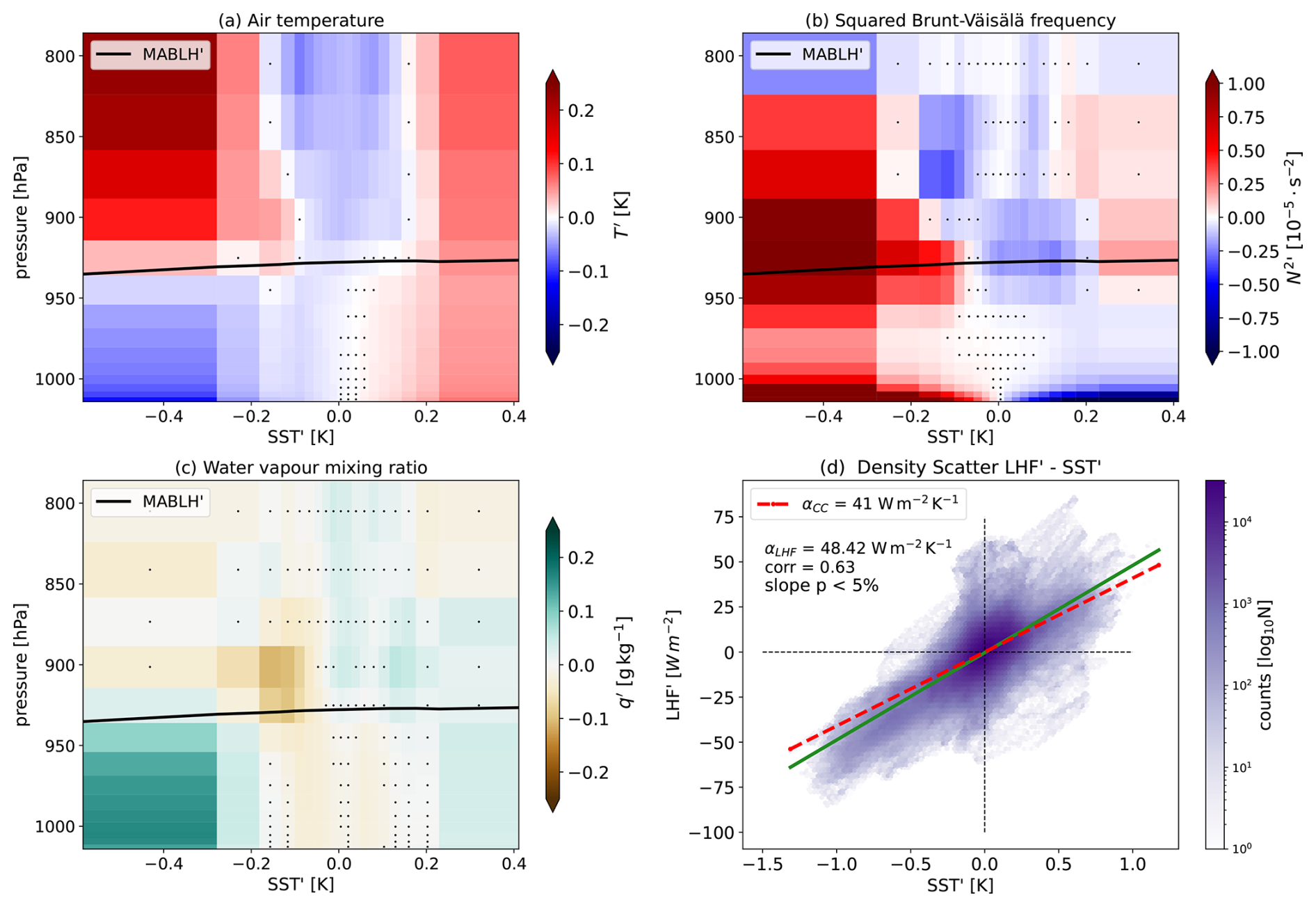
Figure 3 MABL response, in terms of anomalies, of (a) air temperature T, (b) Brunt-Väisäla frequency N², (c) water vapor mixing ratio q. The thick black line represents the bin-averaged MABLH anomalies summed to its monthly-average value. Stippling indicates where results are not statistically significant according to the p value criterion ensuing from the two-tailed Student's t test. (d) Scatter plot and linear regression (light blue solid line) between model-derived surface latent heat flux (LHF) and SST anomalies. The dashed red line indicates the scaling due to Clausius-Clapeyron only (α_CC), centered on the mean SST. The slope of the linear regression, its p value (based on a two-tailed Student t test) and the value of the correlation coefficient (corr) are indicated in the legend.

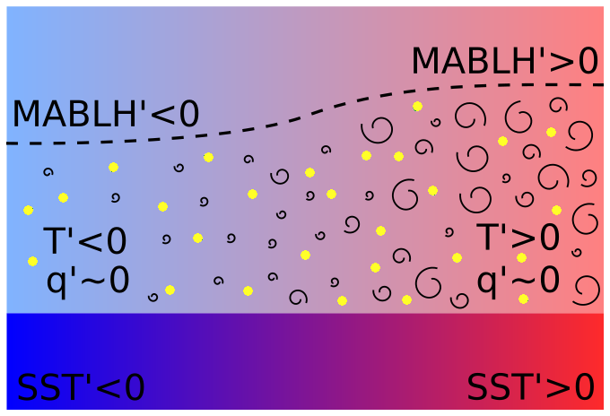
Figure 4 Summary schematic of the main atmospheric anomaly responses. SST^′ are denoted with the colors in the lower part (blue: cold, red: warm). Air temperature anomalies are indicated by the colors in the upper part. The concentration of yellow dots is proportional to MABL humidity anomaly. Whirls number and size indicate the intensity of the atmospheric turbulent mixing, which results in different MABLH^′, as shown by the dashed line.

4 Summary and conclusions

Spatially-varying SSTs significantly impact sensible and latent surface fluxes, with warm (cool) ocean patches heating up (cooling down) and thickening (shrinking) the MABL. The MABL height is modulated by the entrainment at its top (Neggers et al., 2006), which is strengthened over positive SST anomalies and reduced over negative ones following from a tighter control of surface buoyancy production by the locally-enhanced sensible heat fluxes. Overall, MABL humidity anomalies are not substantially modified by fine scale SST anomalies. At the spatial scales considered, O(100–1000 km), the adjustment of MABL humidity due to surface evaporation is counterbalanced by the growth of entrainment fluxes that dry the MABL. The net effect of the MABL top drying, then, is to sustain surface evaporation, by keeping the surface air well below saturation, in agreement with Borgnino et al. (2025). These relationships are depicted in the schematic of Fig. 4. In this terms we argue that moisture is set by large-scale environmental conditions and it is insensitive (or weakly sensitive) to small-scale SST variability. Understanding how surface evaporation behaves at the mesoscale is, nonetheless, important as it has been recently recognized to control the water budget components within the MABL (Giordani et al., 2024).

Our findings agree with what was actually observed during EUREC4A (Acquistapace et al., 2022; Chen et al., 2023) and with similar analyses performed with an atmospheric stand-alone numerical model (Borgnino et al., 2025), which support the validity of our methodology. However, the filter used to separate the large scale fields from the mesoscales partially affects the results of the analysis: at times, the large-scale signal may not be completely isolated leading to spurious signals (ref. Fig. 3 and the related discussion).

More thorough investigations, nonetheless, have revealed the role of submesoscale SST variability in the turbulent redistribution of momentum along the MABL column (e.g. Wenegrat and Arthur, 2018) and in the local modulation of hydrostatic pressure (e.g. Meroni et al., 2022), which we have not taken in consideration here. Small-scale oceanic frontogenesis seems to induce additional competing effects in the atmospheric response which negatively feedback on the mesoscale MABL adjustment processes (Conejero et al., 2025) .

As a future development, we propose a more in depth analysis of the specific mechanisms involved in driving the outlined surface fluxes spatial variability taking into account also the spatial variability of surface wind, which is known to be linked to SST variability (Fernández et al., 2023). Future efforts in the investigation could also look into linking SST patterns with the MABL dynamics in a more quantitative way with the use of bulk models (e.g., Neggers et al., 2006).