Assessing the performance of reanalysis and meso-scale model datasets for onshore wind power modelling in Germany

This study evaluates the performance of several reanalysis and meso-scale datasets (ERA5, CERRA, COSMO-REA6, COSMO-R6G2 and NEWA) in modelling wind power generation in Germany and two of its grid control zones. It is the first detailed analysis of CERRA and COSMO-R6G2 for modelling wind energy generation. For this study, wind speeds from several datasets are used to simulate wind power generation for the years 2017 and 2018. The simulations are then compared to observed power generation data provided by the German transmission system operators (TSOs). The study shows that all investigated datasets overestimate the wind energy production in Germany, with overestimation ranging from 5 % to 45 %. As wind turbines are often placed in particularly windy locations within an area (e.g. ridge of a hill or hilltops), this indicates a significant overestimation of the average wind conditions by the reanalysis datasets. When looking at regional variations between the grid control zones, regional differences were observed. In the TransnetBW control zone, characterised by lower mountain ranges, the overestimation was lower. Correlation was generally high with CERRA and ERA5 showing the highest correlations. In general higher-resolution datasets did not perform better than the lower-resolution ERA5 dataset and in many cases showed a weaker agreement with the observed power generation data. Only in the diurnal cycle CERRA reproduced the observed pattern slightly better than ERA5. The study highlights the importance of considering regional and potentially topography-dependent calibrations of wind speed from reanalysis and meso-scale model datasets for power generation modelling. Among the datasets explored, CERRA and ERA5 provide the best wind speed data for wind power simulations, provided that a (regional) bias correction is applied. Moreover, artificial spikes in the diurnal cycle need to be addressed in both datasets. Due to its slightly better diurnal cycle CERRA has an advantage in capturing the temporal variability.

1 Introduction

Modelling the energy generation from wind turbines is a fundamental aspect of the design of the future energy system. The spectrum ranges from planning of transmission grids to the design of regional energy systems. To generate time series of wind power generation for these different applications, temporally and spatially resolved meteorological data is required. Often reanalysis data is used for this purpose (e.g. Staffell and Pfenninger, 2016; Olauson, 2018; Jourdier, 2020; Hayes et al., 2021). Its main advantage is the geographic coverage as well as spatial and temporal resolution. However, despite significant improvements over the recent past, reanalysis datasets have several shortcomings and uncertainties when used to model wind power generation (e.g. Jourdier, 2020; Ramon et al., 2020). A common problem is that wind speeds from reanalyses can have regional biases. Several studies have found either a significant regional overestimation or underestimation of average wind speeds (or both) depending on reanalysis dataset and region (Dörenkämper et al., 2020; Jourdier, 2020; Hu et al., 2023; Pflugfelder et al., 2024; Wilczak et al., 2024). Moreover, due to their coarse spatial resolution, reanalysis datasets are not able to capture the small scale variations of wind speed in complex terrain (Pauscher et al., 2024; Bär et al., 2026). This is especially important since wind turbines are often built in the windiest locations.

For the purpose of evaluation, reanalysis data are often compared with meteorological measurements (e.g. Kampmeyer et al., 2014; Kaiser-Weiss et al., 2015; Jourdier, 2020; Brune et al., 2021; Spangehl et al., 2023). Near surface wind speed evaluations usually rely on station observation data (Kaiser-Weiss et al., 2015) whereas evaluations in higher heights use data from lidars or tall towers. But these measurements are expensive to generate and are often proprietary. They are, thus, often not available for use in modelling or validation. As a consequence, published results at heights relevant for modern wind turbines – if available – are often limited to single (e.g. Spangehl et al., 2023; Lehneis et al., 2021) or comparatively small numbers of locations (e.g. Kampmeyer et al., 2014; Brune et al., 2021; Wilczak et al., 2024). Especially onshore they are often not representative of the entire existing or future wind turbine inventory of a country or region.

When estimating wind energy production from reanalysis data or forecasting models, usually the modelled wind speeds are modified in the power generation modelling pipeline by way of reduction factors or smoothing the wind turbine power curve (e.g. Staffell and Pfenninger, 2016; Hayes et al., 2021). These corrections are often applied by tuning the power generation modelling pipeline to match country wide production data (e.g. Staffell and Pfenninger, 2016; Olauson, 2018).

In this paper we use a different approach and assess the performance of the reanalysis and meso-scale model datasets to model wind power generation in Germany. For this purpose we compare the freely available datasets ERA5 (Hersbach et al., 2017), CERRA (Schimanke et al., 2021), COSMO-REA6 (Bollmeyer et al., 2015), COSMO-R6G2 (Bär et al., 2026) and NEWA (Hahmann et al., 2020; Dörenkämper et al., 2020). Similar methods have been applied to other dataset combinations in other works. Jourdier (2020) analysed the performance of different reanalysis datasets in France and found differences between datasets but also highlighted regional variations. Murcia et al. (2022) used ERA5, NEWA and EIWR with additional scaling using the Global Wind Atlas. In contrast to Jourdier (2020), they concluded that all datasets showed good performance and highlighted the benefit of finer resolution downscalings. Gualtieri (2022) in a meta analysis of 15 reanalysis datasets found that reanalyses in general and ERA5 in particular are capable in offshore and flat onshore regions but that they show wind speed overestimation in coastal regions and wind speed underestimation in mountainous regions.

In this analysis, we focus on regional differences in Germany and model the generated power using wind speeds from different reanalysis and meso-scale model datasets. Instead of tuning the power curve with fudge factors for losses or correcting the wind speeds with country-wide constant factors, we analyse the biases observed in Germany and different German regions. For this purpose we remove the components of the power generation modelling pipeline that modify the wind speeds and instead account for curtailment due to redispatch and estimated general losses after the annual energy is simulated. Curtailment due to sources other than redispatch are included in the general losses. The simulated power generation time series is then compared to observed power generation. This way, remaining differences should be in large parts due to the performance of the reanalysis and meso-scale model datasets in representing wind speeds. We focus our study on the years 2017 and 2018 due to data availability (see Sect. 2.4).

This approach to some extent causes the risk for a selection bias as wind turbines are not placed randomly but in windy locations where wind speeds are likely higher than the average in the model grid cell. If the model represented average wind conditions an underestimation of energy production would be expected. On the other hand this approach has the advantage of a much better spatial coverage as the number of wind turbines is much higher than that of available measurements. Moreover, the wind datasets are assessed directly on the target application (i.e. power generation modelling) and, thus, do not suffer from biases introduced by differences in site characteristics between wind measurement locations and turbine sites of the wind park portfolio. The paper aims to provide an overview of the strengths and weaknesses of different reanalysis and meso-scale model datasets in modelling the wind power generation in Germany and derive recommendations for their application. For this purpose, the performance with regards to regional as well as the temporal (diurnal) patterns is assessed.

2 Methods

This section details the datasets and modelling approaches that were chosen to facilitate the comparison of wind speed data in reanalysis datasets and the energy production of wind turbines. This entails the description of the model to simulate the energy production as well as its input datasets on the wind turbine characteristics (i.e. wind turbine location data, power curves of the wind turbines). Moreover, a brief overview of the reanalysis datasets and power generation data used as a reference is also given.

2.1 Wind turbine locations and technical parameters

As this study focuses on the German onshore wind farm portfolio the Marktstammdatenregister (MaStR, Bundesnetzagentur, 2019) provides the most detailed freely available information on the technical specifications of the installed wind turbines. This database is provided by the German grid authority (Bundesnetzagentur, BNetzA) and contains standardised information on each individual turbine. The following parameters are used in this analysis: geographic coordinates, hub height, rotor diameter, installed capacity and commissioning date.

While there is a legal obligation to report data on wind turbines in the MaStR, some turbines are exempt from these obligations and several errors and inaccuracies are present in the database. This requires several post processing steps to improve the quality of the turbine data:

• due to data protection guidelines of the BNetzA, systems with less than 30 kW of installed capacity do not have their geographic location publicly available. These systems are removed from the analysis as their overall impact is limited due to their small size,

• systems with more than 30 kW installed capacity that do not have geographic coordinates, hub height, rotor diameter or installation year associated were removed,

• the specific power (defined as nominal power in Watt divided by the swept rotor area in square meters) is used as a data quality indicator and systems below 180 W m⁻² and above 610 W m⁻² are removed as well. The thresholds are set by the authors based on an analysis of the wind turbine database from Pierrot (2024) and designed to exclude systems with likely unrealistic rotor/generator sizes. The limits only have a very limited impact on the number of removed systems. This is likely due to low quality entries being removed in the prior steps of the clean-up.

In Table 1 the number of removed systems as well as the overall removed capacity is displayed. The dataset was obtained in July 2024 and after clean up, the systems which were operational in 2017 and 2018 are extracted for use in the power generation simulation.

Table 1 Overview of MaStR as of July 2024 and systems removed in quality control. The last two rows show the subset of turbines that are used in the simulations.

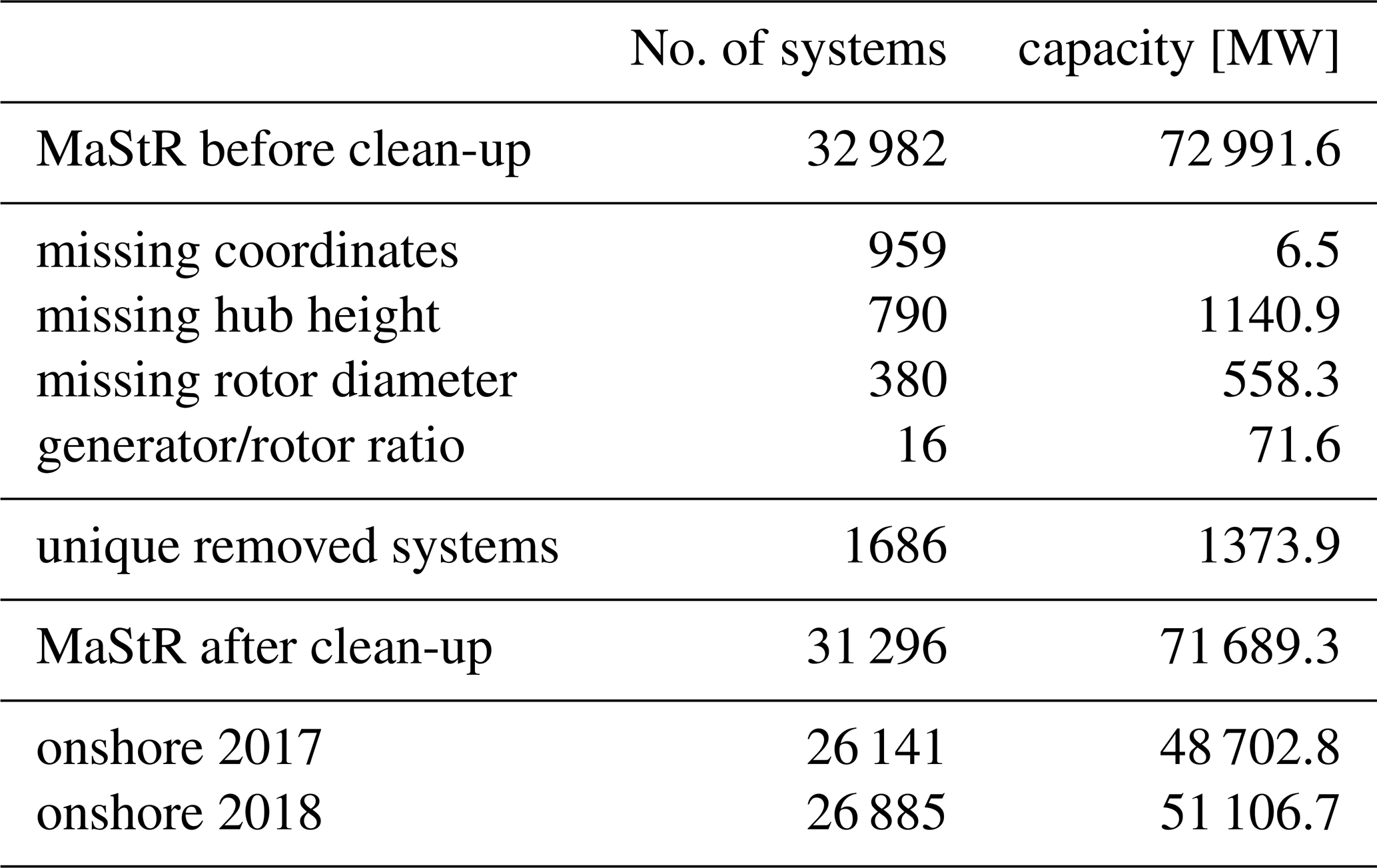
In total 1686 wind turbines are removed due to data problems totalling 1.37 GW. This is around 1.7 % of the total installed capacity of 73 GW. In the subsequent analysis, offshore systems are removed and the remaining systems are further subset by commissioning year. This way the simulated wind turbine portfolio only includes onshore systems operational in the year of analysis. For 2018 this results in 26.885 systems with 51.1 GW. Even with this clean-up there remains a discrepancy between the MaStR data and the reference dataset, which is covered in Sect. 2.3.

This study also investigates the power generation for the control areas of the transmission system operators (TSOs) in regional comparisons. The associated control area for each wind turbine is assigned by its geographic location. A few remaining systems that could not be matched automatically were assigned manually.

Table 2 Details on the wind turbine portfolio installed in the grid zones of the four transmission grid providers in Germany (DE): TransnetBW (TBW), 50 Hertz (50 Hz), Amprion (AMP) and TenneT (TNT) in 2018. Given heights are the turbine site heights in meters, the capacity is given in GW.

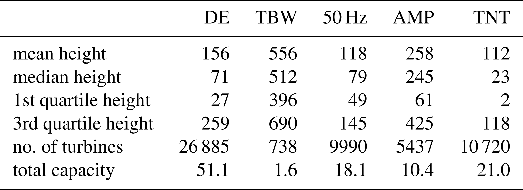
Table 2 shows the ground height above sea level (a.s.l.) and power distribution of the wind turbines for Germany as well as the control areas. The height above sea level is used in the later analysis as a proxy for terrain complexity and exposure of the turbines as high terrain tends to also be complex in Germany.

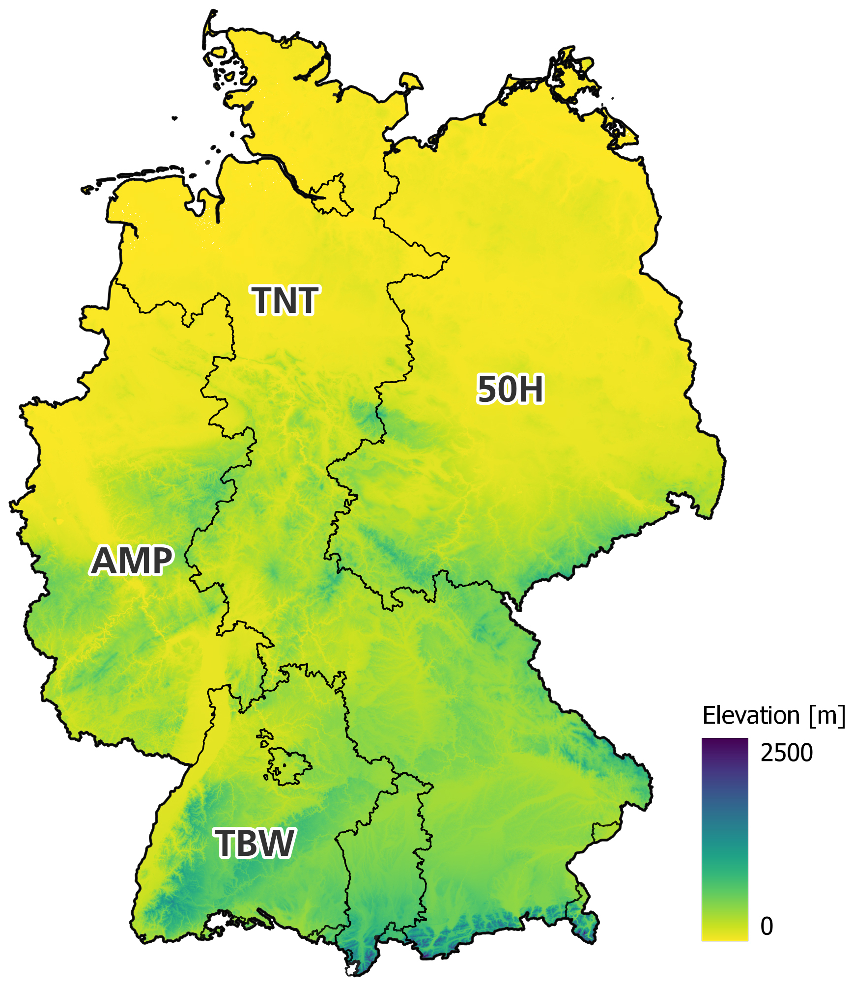
Figure 1 Map of Germany highlighting the control areas of the TSOs as well as the terrain elevation. © BKG (2018) dl-de/by-2-0.

As can be seen from Table 2, the turbines in the TransnetBW (TBW) control area are mainly located in complex terrain, while the 50 Hz control area (50 Hz) mainly contains turbines in flat terrain. Therefore, these two regions represent well the range of regional variations in terms of terrain complexity and turbine elevation. This makes TBW and 50 Hz good candidates for investigating regional and topographical effects and biases in wind power modelling from reanalyses and meso-scale models. For this reason, this study focuses on these two control areas in addition to the whole of Germany.

2.2 Methodology for Generating Synthetic Power Curves

To be able to compare reanalysis and meso-scale models with power generation data the simulated wind speeds need to be converted to generated power. The cornerstone of this approach is a power curve model that generates a power curve for each individual turbine. Since MaStR does not contain power curves directly, a generic model to generate synthetic power curves is used. In contrast to the approach by Saint-Drenan et al. (2020), a power coefficient (c_p) characteristic curve is not analytically derived from parameter values; rather, synthetic characteristics of the power curves are interpolated based on real power curve characteristics. This method has the advantage that it accounts for the differences between the power curves of high and low speed turbines, and it allows for addressing performance- or manufacturer-specific characteristics (such as cut-in wind speed, ramp up and cut-out wind speed).

A systematic methodology is employed to generate synthetic power curves from empirical data. Power curve profiles from the TheWindPower database (Pierrot, 2024) are first filtered for plausibility and subsequently clustered based on specific power density characteristics. The profiles are categorized into multiple turbine categories according to their operational wind regimes, with characteristic reference curves derived through cluster averaging. Synthetic power curves are then generated by scaling the reference curves to target power density specifications using the cubic relationship between power density and wind speed.

Starting from the fundamental wind power equation, we assume that the power coefficient c_p remains constant with respect to wind speed and that air density is also considered constant. Consequently, the cube of the wind speed v³ is proportional to the power P divided by the rotor area A, which leads to the definition of specific power density as a relevant reference metric shown in Eq. (1):

$$\begin{array}{}\text{(1)}& P\propto A\cdot v^{\mathrm{3}}\text{ and }v\propto \sqrt[\mathrm{3}]{{\displaystyle \frac{P}{A}}}\end{array}$$

Equation (2) shows that the wind speeds of the generic curve v_a and the reference curve v_b are related by the cube root of their respective specific power densities:

$$\begin{array}{}\text{(2)}& {\displaystyle \frac{v_{\mathrm{a}}}{v_{\mathrm{b}}}}=\sqrt[\mathrm{3}]{{\displaystyle \frac{{\frac{P}{A}}_{\mathrm{a}}}{{\frac{P}{A}}_{\mathrm{b}}}}}\text{ and }{v}_{\mathrm{a}}=v_{\mathrm{b}}\cdot \sqrt[\mathrm{3}]{{\displaystyle \frac{{\frac{P}{A}}_{\mathrm{a}}}{{\frac{P}{A}}_{\mathrm{b}}}}}\end{array}$$

v_a: Wind speed of the model power curve [m s⁻¹]; v_b: Wind speed of the reference power curve [m s⁻¹]; ${\frac{P}{A}}_{\mathrm{a}}$: Specific power density model power curve [W m⁻²]; ${\frac{P}{A}}_{\mathrm{b}}$: Specific power density reference power curve [W m⁻²].

This scaling relationship enables the generation of synthetic power curves for any desired specific power density, providing a robust and generic modelling approach that is independent of IEC turbine classes or manufacturer-specific technical characteristics.

2.3 Wind energy production data

For the evaluation of simulated power generation using wind speeds from reanalysis and meso-scale model datasets, we use wind power generation data from the electricity and gas market data (Strom- und Gasmarktdaten, SMARD) portal of the BNetzA (Bundesnetzagentur, 2025). From the available datasets, power generation from onshore wind farms for all of Germany as well as data for the control areas of the TSOs is used. Wind energy production is available as 15 min sums which are re-sampled to hourly resolution to match the repreanalysis datasetsmodelled wind power production.

SMARD also provides the installed capacity for each year. A comparison with MaStR revealed that there are small differences between the installed capacity calculated from the MaStR and the value given in the SMARD data. In 2017 SMARD has around 1.6 GW (3.3 %) less installed capacity than the value calculated from the MaStR. In 2018 the installed capacity is 0.6 GW (1.2 %) higher for SMARD than for the MaStR. To account for the differences the model output is scaled by the differences between the two datasets. The SMARD data only includes the observed power generation. Curtailment and other losses are therefore implicitly included in these data, while the modelled power generation does not account for curtailment due to redisptach and other losses. The raw simulations are therefore reduced by the curtailment due to redispatch reported by Borrmann et al. (2020).

As Borrmann et al. (2020) gathered data describing curtailment due to redispatch by state, an assignment to control areas is only possible where the control area border aligns with the state border. This is the case for the TBW control area as it matches the border of Baden-Württemberg. The same is true for the 50 Hz control area which encompasses the states in Eastern Germany and Hamburg.

In a final step losses in the energy production have to be considered. These include aerodynamic losses due to wake effects, sector management, curtailment because of noise emissions and shadow flicker, curtailment for reasons of wildlife protection (birds and bats), losses due maintenance and unplanned downtime as well as electrical losses in the wind farm grid. In energy system modelling losses are often accounted for by modifying the power curve (e.g. Staffell and Pfenninger, 2016; Hayes et al., 2021) and/or applying wind-speed dependent loss functions (e.g. Pflugfelder et al., 2024; Hayes et al., 2021). However, this makes it difficult to objectively compare the simulated and observed power generation and to compare different wind data sets, as the power curves can always be tuned to match the observed power production. We therefore chose a different approach here and estimate the losses as a percentage of the simulated production. For Germany we use the losses of 12.5 % of the energy production. These numbers are derived from expert guesses of several project developers and wind energy consultants operating in Germany and a series of (confidential) resource assessments for wind farms in Germany. We acknowledge this number to be somewhat subjective but deem it more transparent than modifying the power curves. To give an indication of the uncertainties in our estimates we also provide whiskers in the analysis indicating a variation of 7.5 % to 17.5 % losses.

2.4 Reanalysis datasets

For the presented analysis we use five modern reanalysis and meso-scale model datasets. In general we use wind speeds from the analysis run, except for CERRA where a combination of analysis and forecast runs is used. ERA5 (Hersbach et al., 2017) is a global reanalysis dataset provided by ECMWF with a horizontal resolution of ∼31 km. This dataset is frequently used in many different fields and therefore well established as a baseline in energy systems analysis. It provides global coverage, hourly resolution and showed a good performance in other evaluations e.g. Olauson (2018) and Brune et al. (2021). In this paper we use the dataset provided by the Copernicus Climate Datastore which is delivered as a regular 0.25° × 0.25° grid interpolated from the original reduced Gaussian grid.

CERRA (Schimanke et al., 2021) is a European downscaling of ERA5 with a horizontal resolution of ∼5.5 km. It covers Europe with hourly resolution and in comparison to other reanalysis systems it uses a combination of 3-hourly analysis/assimilation runs which are extended for 6 h using a forecast model. One can obtain an hourly time series by combining the analysis with different forecast lead times. For this analysis two different wind speed datasets are created from the CERRA raw data. CERRA-short uses each of the analysis steps in combination with the +1 and +2 h steps of the forecast model. CERRA-long uses only forecast data from the lead times +3 to +5 h. We use both combinations, CERRA-short and CERRA-long in the following analysis.

COSMO-REA6 (Bollmeyer et al., 2015) is the regional reanalysis of the German weather service (DWD) with a horizontal resolution of ∼6.6 km. It covers Europe with hourly resolution and is a regional downscaling of ERA-Interim (Dee et al., 2011). Production has stopped due to the discontinuation of ERA-Interim and the data is available up to mid 2019.

The DWD is currently producing the successor to COSMO-REA6, COSMO-REA6 Generation 2 (R6G2) (Bär et al., 2026). It has the same spatial and temporal resolution as COSMO-REA6. It uses an updated version of the COSMO model and is driven by ERA5 instead of ERA-Interim. A first comparison between the two datasets by Bär et al. (2026) indicated similar wind speeds for COSMO-REA6 and COSMO-R6G2 but also regional differences especially at night time.

Finally meso-scale simulations of the New European Wind Atlas (NEWA) (Hahmann et al., 2020; Dörenkämper et al., 2020; Hahmann et al., 2021; Syed and Mann, 2024) are evaluated. With a horizontal resolution of about 3.3 km they have the finest spatial resolution. The NEWA meso-scale simulations were created by downscaling ERA5 using the forecasting model WRF. In contrast to the reanalysis systems, no data assimilation is performed in the modelling domain.

For CERRA, COSMO-REA6 and NEWA the wind speed time series are extracted from the products that provide height levels above ground level. For COSMO-R6G2 a lookup table provided by DWD is used to match model levels to their corresponding height. To simulate the wind speed at the turbine (hub) height, wind speeds in the closest levels above and below each wind turbine's hub height are used and wind speeds are then interpolated to hub height using the power law. The ERA5 dataset does not provide wind speed directly, instead it has to be computed from the U- and V-components. These in turn are not provided on height levels (except at 10 and 100 m) but instead on model levels. To find the model level at a given altitude the geopotential height has to be used which can be computed from the geopontential. The geopotential is included in the dataset, however, it is only archived on the first model level. Using the logarithm of surface pressure and the geopotential at the surface as well as temperature and humidity on model levels, the geopotential for each model level can be computed. The altitude of the model level is then computed via the geopotential height. The U and V components are extracted for the model levels that are above and below the given hub height and interpolated to hub height. The reader is referred to ECMWF (2025) for additional information on the process. For all models the grid cell where the wind turbine is located is selected using a nearest neighbour comparison of the turbine coordinates and the centroid of the grid cell.

3 Results and discussion

In this section, we first evaluate the reanalysis and meso-scale model datasets by comparing the simulated total energy production with the observed energy production. This includes a regional analysis based on the TSO control areas as well as an analysis of the distribution of production differences. Following this, we perform an assessment of the underlying models’ ability to capture temporal variations. For this purpose, we first carry out a correlation analysis of power generation using the time series data of power production. We then investigate the models' ability to capture the diurnal cycle of energy production. In Sect. 3.1 we use yearly curtailment data and estimation of losses to correct the total simulated energy production. All other analyses use the simulation results without correction for losses and curtailment as they are based on hourly data. Time series of curtailment and losses were not available.

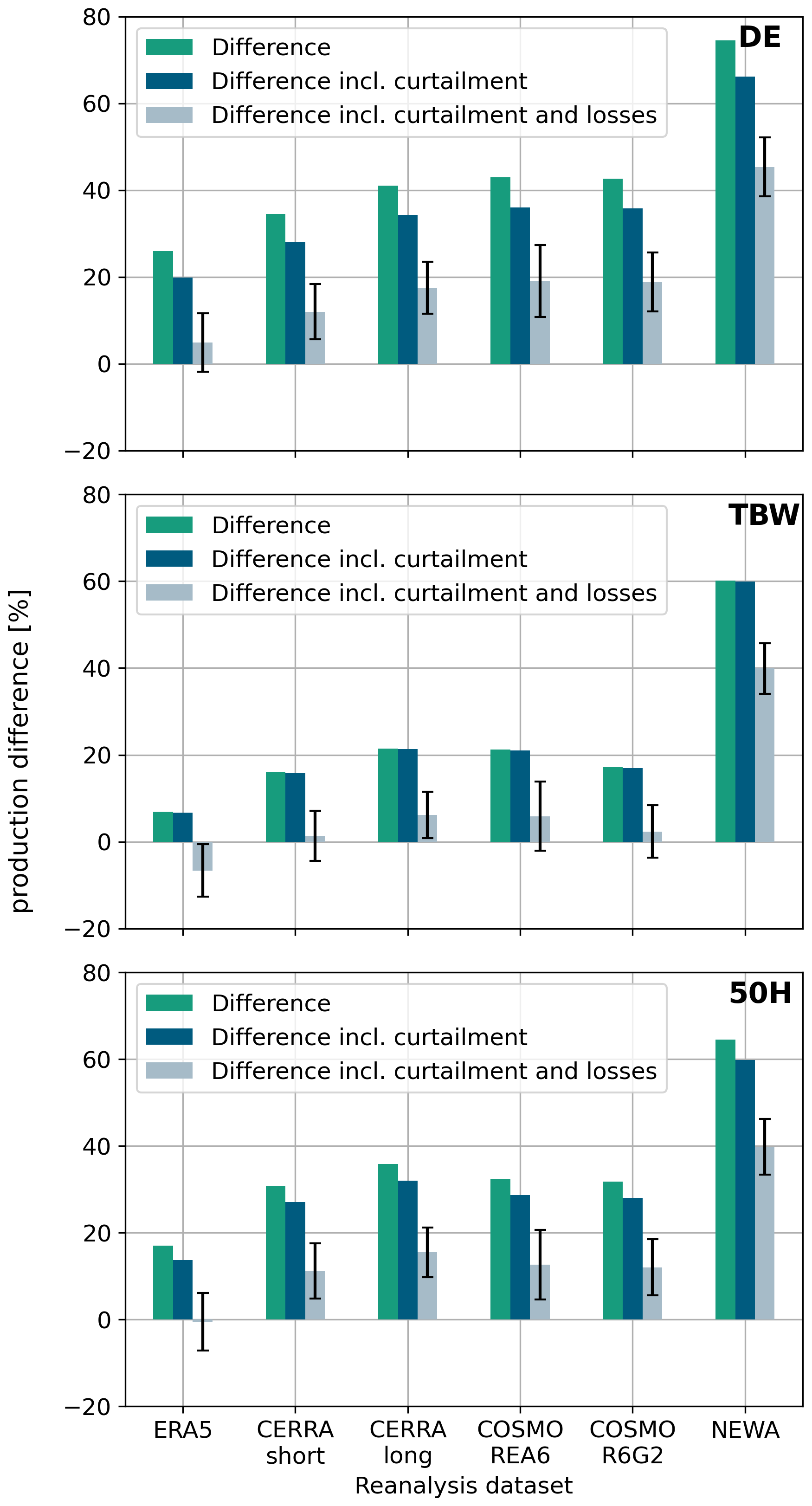
Figure 2 Differences in annual wind energy production between the SMARD data and different reanalysis datasets for Germany (DE), the TransnetBW control area (TBW), and the 50 Hz control area (50 Hz) in 2018. Differences are shown for raw production (green), accounting only for curtailment due to redispatch (blue) and accounting for curtailment due to redispatch and losses (grey). The black whiskers indicate a variation of ∓5 % in the estimated losses.

3.1 Annual energy production

Figure 2 shows the annual production difference in wind energy as measured by SMARD in comparison to the simulated energy production using the different reanalysis and meso-scale datasets for 2018. It also illustrates the effects of incorporating the corrections for curtailment due to redispatch and losses. The comparison is shown for Germany (DE), the TransnetBW control area (TBW), and the 50 Hz control area.

The first bar (dark green) illustrates the difference in energy production without any corrections, the second bar (dark blue) depicts the impact of curtailment due to redispatch, and the third bar (light blue) represents the combined effects due to redispatch and losses. The whiskers in all plots indicate the range of losses, which spans from 7.5 % to 17.5 %, with a midpoint of 12.5 % represented in the light blue bar. The whiskers therefore provide an indication associated to the estimation of the losses. We acknowledge that this is somewhat subjective.

The top panel (DE) shows the results for all wind turbines in Germany. For Germany, all datasets exhibit an overestimation of production. ERA5 shows the closest match to the production from the SMARD data. The overestimation of approximately 5 % is in the order of the assumed uncertainties for the production losses. CERRA-short and CERRA-long show a similar performance (12 % and 17 % overestimation). Notably, only changing the forecast lead times causes a difference of approximately 5 % between the two CERRA datasets. COSMO-REA6 and COSMO-R6G2 are very similar and exhibit an overestimation of approximately 19 %. NEWA presents by far the highest overestimation which is more than double than that of COSMO-REA6 and COSMO-R6G2 at 45 %.

The observed overestimation of energy production and its variation across all datasets highlights that energy systems analysis requires additional careful and dataset specific corrections. Interestingly, the dataset with the coarsest resolution (ERA5) shows the best match with the SMARD data. The deviations in the finer scale datasets CERRA, COSMO-REA6 and COSMO-R6G2 are approximately 2.5 to 4 times higher than ERA5. NEWA, the dataset with the finest resolution, shows by far the highest deviation. These results strongly suggest that increasing the horizontal resolution of the underlying models does not automatically reduce biases in wind speed on a country-wide scale.

In this context it is also important to note that wind turbines are usually constructed in locally windy areas. The overestimation of the average wind speed and in turn the wind energy resource in the respective grid cells of the underlying models is likely to be greater than suggested by Fig. 2. Thus, the observations indicate an overestimation of the wind resource across all models.

The middle panel (TBW) presents the same analysis for the TransnetBW control area (Fig. 1). TBW is characterized by complex terrain with an average wind turbine elevation of 560 m above sea level (refer also to Table 2). In this region, the differences between the SMARD observations and the power generation model outputs diverge significantly from the Germany-wide results. Although there remains an overestimation in both the raw results and those including curtailment due to redispatch, incorporating losses results in an underestimation of the annual energy production in the control zone for ERA5 by approximately 7 %. Both CERRA datasets show a significantly lower overestimation of the annual energy production for TBW than for DE, with their difference being similar to that observed in DE. While COSMO-REA6 and COSMO-R6G2 also have a lower overestimation in TBW they are no longer similar with COSMO-R6G2 now showing less overestimation than COSMO-REA6. The differences are in line with the observation of (Bär et al., 2026) that COSMO-R6G2 shows lower wind speeds in hilly exposed locations. Bär et al. (2026) attributed this mainly to lower nocturnal maxima in the wind speeds at elevated heights.

NEWA continues to exhibit the highest level of overestimation among the datasets. For TBW, this overestimation is approximately 40 %. Interestingly, this is the smallest difference between DE and TBW across all evaluated models. This might hint at some advantages of the fine resolution in better capturing topography-induced differences.

The bottom panel (50 Hz) illustrates differences between the simulated wind energy production and the SMARD data for the 50 Hz control area. This control area predominantly features flat terrain with an average turbine foundation height of 118 m above sea level. In this region, the overestimation of energy production compared to Germany (DE) is reduced. ERA5 exhibits an underestimation of 1 %, while CERRA-short and CERRA-long show 11 % and 15 % overestimation. With a 12 % overestimation, both COSMO-R6G2 and COSMO-REA6 show the largest reduction in overestimation for 50 Hz. For NEWA the numbers are very similar to TBW.

Overall, the analysis of wind energy production reveals notable differences between different datasets and regions. Some of them are likely to be connected to the orography in the investigated areas. For example, in the TBW control zone, wind turbines are predominantly placed on lower mountain ranges. In this terrain, local variations in wind speeds are higher than in flat areas. The power generation from the SMARD data is likely to represent wind conditions on hill tops and ridges with exposed and (locally) windy conditions. While the good match of the simulations from many of the reanalysis datasets for TBW is positive for wind power generation modelling, it also indicates that the average wind conditions in the grid cells are likely not well represented by the underlying models. While also true for DE and 50 Hz this effect is likely to be less pronounced there because the average terrain complexity of the turbine locations is lower.

Our results are consistent with those of Jourdier (2020) and Gualtieri (2021), where ERA5 showed underestimation in complex terrain and overestimation in flat terrain. In their analysis, higher resolution models such as COSMO-REA6 performed better in complex terrain. While we also find reduced biases for CERRA and COSMO-R6G2 in our analysis, a comparison of the wind park portfolio suggests that the characteristics of turbine locations also significantly differ between more complex and flatter areas. In more complex terrain, turbines tend to be more exposed with locally more windy conditions. We therefore suspect that the selection bias towards windy locations is stronger in the TBW area. In this scenario the observed reduction in the biases in the finer scale datasets is not caused by a better ability to resolve local wind conditions. It is merely the result of the compensating effects of the bias in the estimation of the representative wind speeds by the underlying models and the selection bias introduced by the wind turbine placement. This is further supported by the observation, that the differences in production bias between DE and TBW are very similar for ERA5 and CERRA. This effect could be mitigated by enriching coarser scale reanalysis and meso-scale model datasets with local topographically induced influences and removing biases by applying data driven corrections from spatially distributed wind measurement networks (Hu et al., 2023, e.g.). Ideally, these should include wind turbine hub heights which are of interest for wind energy applications.

In our analysis, NEWA showed high overestimation in all cases. This is in in line with the results of Murcia et al. (2022), where modelled country-wide capacity factors based on wind speeds from NEWA were shown to be much higher compared to observed capacity factors. While the German capacity factors were not listed explicitly, all countries were shown to have overestimation to varying degrees. Our analysis is also in line with findings of Jourdier (2020) where NEWA is shown to consistently overestimate both wind speed and wind turbine energy production. A comparison of the results for 2018 to 2017 reveals that the general patterns are very similar (Fig. A1). However, the observed power production is higher in comparison to the modelled power production leading to slightly reduced production differences. For DE, the production differences are approximately 2 % to 5 % smaller. For TBW, the production difference in 2017 is 2 % to 8 % smaller compared to 2018. In the 50 Hz control area, the production difference in 2017 is approximately 1 % to 7 % greater than in 2018. For DE and TBW both CERRA datasets show the largest change, while for 50 Hz the COSMO datasets show the largest change. The changes in the differences indicate that – while the wind park portfolio was similar between both years – the performance of the investigated datasets in simulating different years might vary. A systematic analysis of the performance over several years should be carried out in the future. However, due to potential effects of the changing wind farm portfolio, this is beyond the scope of this paper.

3.2 Distribution of production difference

The distributions of the normalized hourly power production difference for all datasets in Germany (DE) and TransnetBW control area (TBW) are shown in Fig. 3. The production difference is normalized by the average hourly power production to ensure consistency with Fig. 2. To convert this into power production difference normalized by installed capacity, the values on the x axis need to be multiplied by 0.196 and 0.199 (capacity factors of DE and TBW). In general, all datasets show high occurrences of differences between −25 % and 25 % and almost no differences smaller than −25 % in DE. ERA5 is showing by far the highest occurrences of small differences, which is expected given the results from Sect. 3.1. With increasing difference, the occurrence decreases, and there are almost no differences larger than 125 % for ERA5. Both CERRA datasets show a similar pattern although they do have fewer occurrences of small differences compared to ERA5. Their drop off is also not as fast as for ERA5 for larger differences resulting in higher total overestimation. Compared to CERRA-long, CERRA-short shows more occurrences between −25 % and 25 % and fewer occurrences between 25 % and 75 %, and 75 % and 125 %. This is likely due to spikes of lower simulated production which can also be observed in the diurnal cycle (see Sect. 3.4). COSMO-REA6 and COSMO-R6G2 show almost identical distributions and both exhibit a reduction of occurrences with increasing difference. However, compared to ERA5 and CERRA, they have notable occurrences at 125 % to 175 % difference. The distribution of the differences is significantly flatter for NEWA and more occurrences at higher differences can be observed. Interestingly, NEWA also has a substantial number of occurrences at more than 125 % and even a significant amount of differences of more than 175 % can be observed.

In the TBW control area, the distributions are a slightly more centred than in DE, and more negative differences can be observed. The occurrence of small differences has increased substantially in all datasets except ERA5 where the picture is similar to that in DE. Both CERRA datasets now show almost as many occurrences at −25 % to 25 % as ERA5 and more than COSMO-REA6 and COSMO-R6G2 in this bin. CERRA-long still shows more occurrences than CERRA-short but the difference has decreased. Differences higher than 25 % are significantly reduced for TBW. Between the datasets, similar patterns as for DE can be observed for TBW. Among the datasets, ERA5 and COSMO-R6G2 show the most occurrences for stronger negative deviations below −25 %, followed by COSMO-REA6 and both CERRA datasets. NEWA shows the fewest occurrences of all models for this bin. Notably, some negative deviations for the bin smaller than −75 % can be observed for TBW. Again, the largest numbers in this bin are found for ERA5, COSMO-REA6 and COSMO-R6G2. The 50 Hz control area is omitted, as the results are very similar to DE.

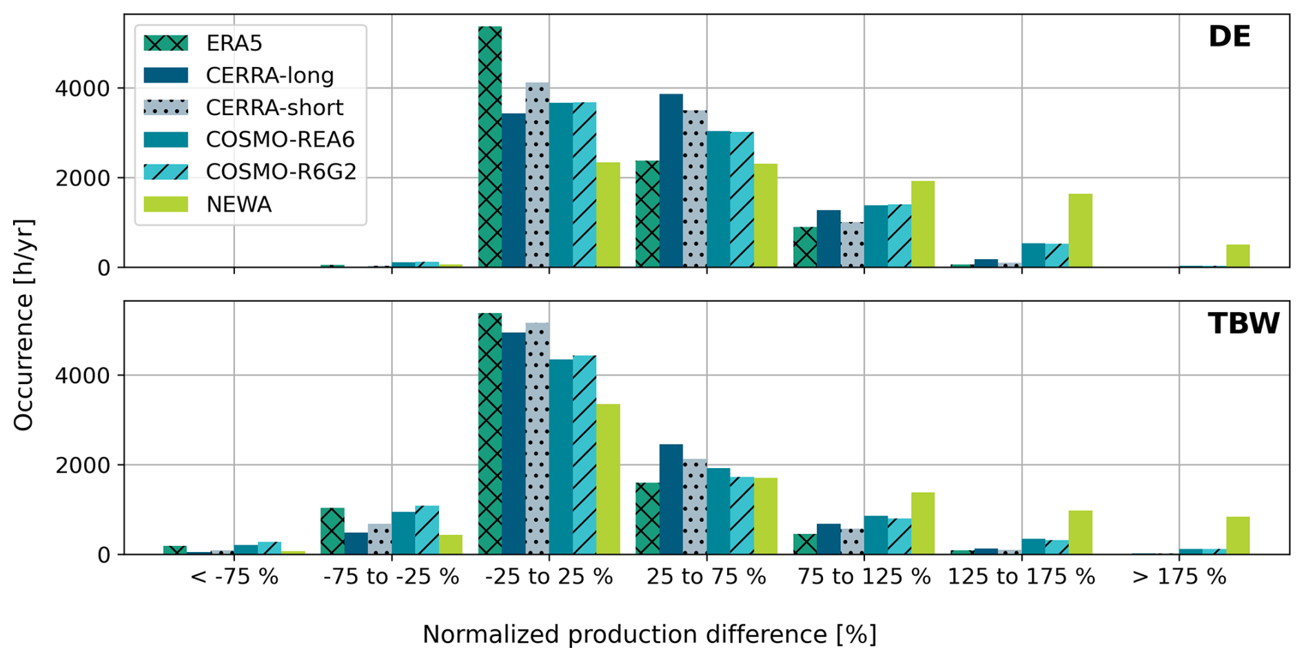
Figure 3 Distribution of the occurrence of normalized production difference for 2018 in DE and the TBW control area. The differences are normalized with the average of measured yearly production. To convert this into differences normalized by installed capacity, the values on the x axis need to be multiplied by 0.196 and 0.199 (capacity factors of DE and TBW).

3.3 Correlation analysis

To evaluate the performance of the datasets in capturing temporal variations, we analyse the correlation between observed and modelled energy production. Figure 4 illustrates the correlations between the SMARD data and the simulations in three panels representing Germany alongside the TBW and 50 Hz control areas. In this figure, green squares represent data from 2017, while orange dots correspond to 2018.

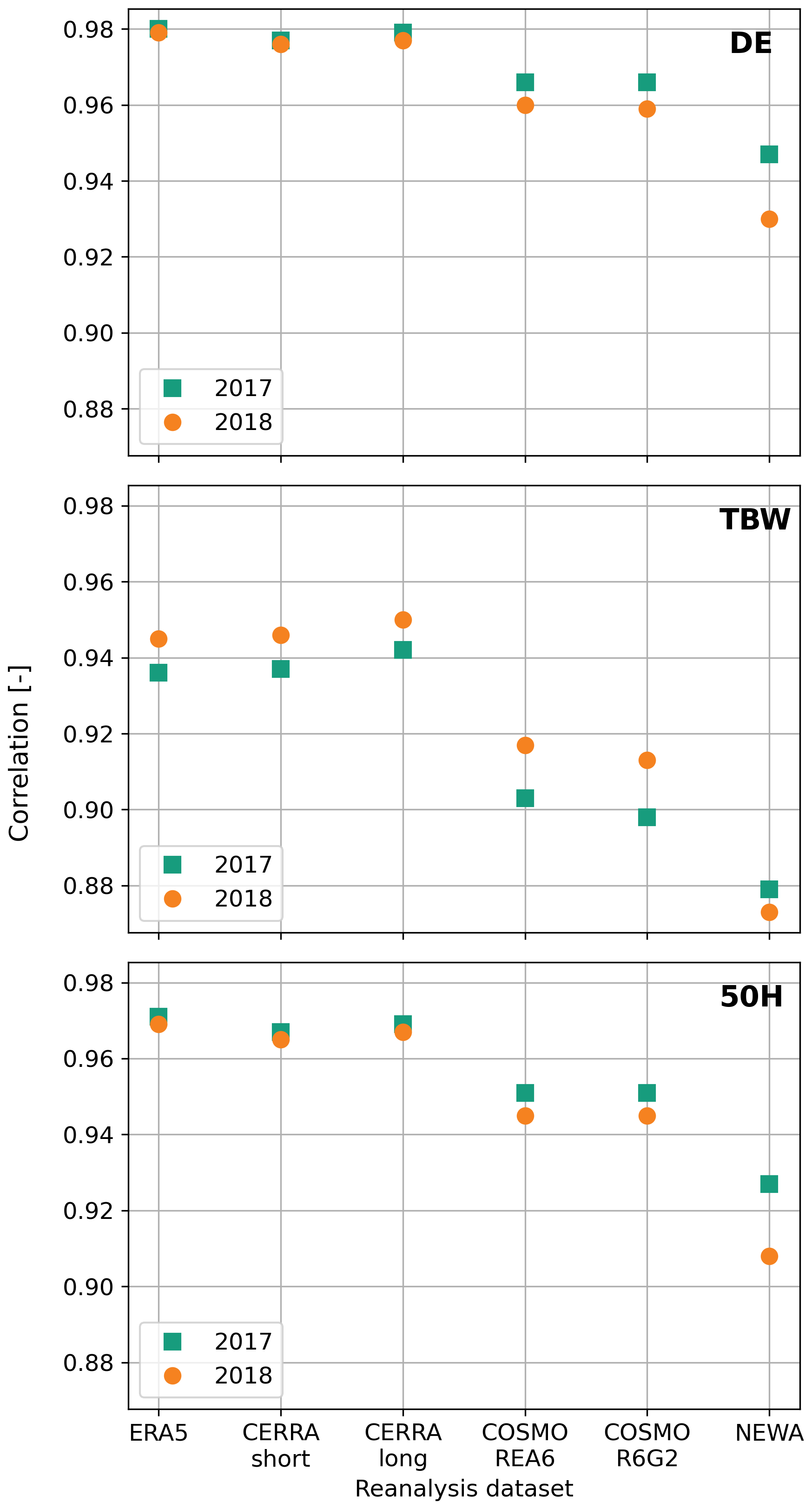
Figure 4 Correlation between observed wind energy production and simulated wind energy production for Germany in 2017 and 2018 for the models ERA5, CERRA-short, CERRA-long, NEWA, COSMO-REA6 and COSMO-R6G2.

The simulated power production from ERA5, CERRA-long and CERRA-short demonstrates very similar and very high correlations with values close to 0.98, exhibiting minimal year-to-year variation. COSMO-REA6 and COSMO-R6G2 show slightly lower correlations having values close to 0.96. They also exhibit marginally greater variation between the years. NEWA has the lowest correlations, ranging from 0.93 to 0.95, alongside higher variation between the years. The lower correlations in COSMO-REA6 and COSMO-R6G2 might be caused by different physical parametrisations or data assimilation methods. However, they are probably in part due to the underlying models' inability to properly capture the diurnal patterns in power production (Sect. 3.4). The significantly worse correlation of NEWA is likely caused by the fact that NEWA did not use data assimilation in the modelling domain. It has previously been reported to show weaker performance in capturing temporal variations (e.g. Spangehl et al., 2023). The country-wide correlations for ERA5 and NEWA are in alignment with Murcia et al. (2022) where they found very similar correlations for Germany. Jourdier (2020) showed similar results for France with ERA5 outperforming the other datasets, closely followed by COSMO-REA6. NEWA showed the lowest correlation.

In the TBW control area, the middle panel reveals that the correlation of observed versus modelled wind energy production is generally lower than that for all of Germany, yet inter-dataset differences remain similar. Correlations for CERRA-long are slightly higher than for ERA5. This might indicate CERRA's ability to better capture variations in complex terrain. However, the differences are very small. Both COSMO-REA6 and COSMO-R6G2 exhibit lower correlations and slightly higher variation between the investigated years. NEWA is again the worst performing dataset with correlations below 0.88. The influence of complex terrain is also shown by Jourdier (2020) where locations in mountainous regions show a reduction in correlation across all investigated datasets.

The bottom panel (50 Hz) illustrates correlations for the 50 Hz control area. Similar to the energy production analysis, correlations are lower when compared to the national results but show higher correlations when compared to the TBW control area.

The lower correlations found in TBW might be caused to some extent by the fact that meso-scale models fail to appropriately resolve micro-scale effects, which are more important in complex orography. However, a large part of the differences in correlation is likely caused by the differences in the number of turbines (Table 2) and spatial extent (Fig. 1). TBW has less than one tenth of the number of turbines compared to 50 Hz. DE has approximately 2.7 times the number of turbines compared to 50 Hz.

Comparing the correlations from the different datasets, no clear trend between horizontal resolution and correlation can be identified. The reproduction of the diurnal cycle on the national and the control zone level seems to be more dependent on other factors like data assimilation methods.

To give more detailed insights into the correlations, Fig. 5 shows scatter plots of the observed and simulated power production for selected datasets for Germany and the TBW control area as hourly, daily and monthly averages. The relationship of the simulated and observed power generation seems to follow a more or less linear relationship for ERA5 (left column in Fig. 5). For COSMO-R6G2, a slightly more curved shape can be observed (middle column Fig. 5). This behaviour is even stronger for NEWA (right column in Fig. 5). Especially for TBW, NEWA shows a strong curvature and the highest overestimation around the middle of the observed power production range on average. The daily and the monthly values generally follow the same trends with the monthly values only covering the lower range of observed and simulated energy production (as expected). One influencing factor could be the power curve. The produced power has the highest sensitivity to wind speed for medium wind speed ranges between the cut-in wind speed and the wind speed when rated power is reached. However, this effect should be reflected for all datasets, since the power curves used in the simulations are identical. Another explanation could be that the bias in wind speed in NEWA – and to some degree in COSMO-R6G2 – is wind speed dependent. Since this study does not analyse wind speed measurements but power generation, the cause for the curved shape cannot be answered unambiguously. Further analysis comparing wind speeds directly should be carried out. The observation that ERA5 and CERRA (see Fig. B1) show a mostly linear relationship between observed and modelled power production means that a simple scaling function or linear function on power production could yield a simple, good first correction approach. For COSMO-R6G2 and especially for NEWA the quality of this simple approach would likely worsen significantly because of the non-linear relationship indicated by the scatter plots. Applying a linear correction function was not evaluated in this study.

As indicated by the correlations in Fig. 4 the scatter for the hourly values is largest for TBW (see middle row in Fig. 5), which has the most complex orography. However, it should be noted that the installed capacity is about an order of magnitude smaller than for 50 Hz. Also, TBW covers the smallest area out of the analysed zones. These properties are likely to introduce some additional scatter to the potential complex terrain effects. DE, with the largest area and the highest installed capacity, has the lowest scatter. Daily values show similar trends in scatter as hourly values, but the scatter is significantly reduced (as expected). Monthly values only cover the lower production range with little scatter.

While differences in the scatter plots are very pronounced between DE and TBW, the 50 Hz control zone (bottom row of Fig. 5) shows similar behaviour when compared to DE. CERRA-short and CERRA-long have a very similar shape in the scatter plots as ERA5 in all analysed regions. COSMO-REA6 is very similar to COSMO-R6G2 in all analysed regions. Scatter plots for these datasets are shown in Fig. B1).

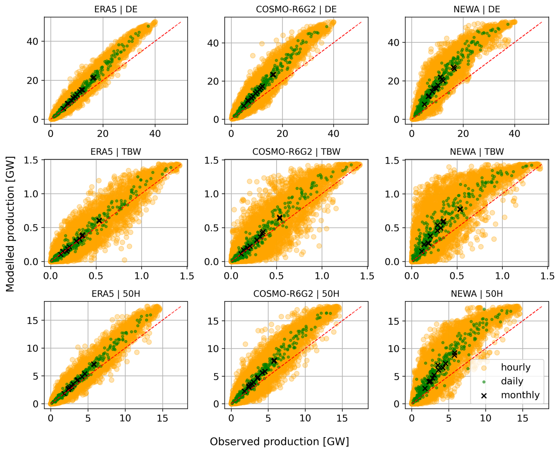
Figure 5 Scatter plots comparing simulated and observed hourly, daily and monthly averaged power production for 2018 for ERA5, COSMO-R6G2 and NEWA for different grid zones and Germany (DE). The dashed red line indicates the 1:1-line. Scatter plots for CERRA-long, CERRA-short and COSMO-REA6 can be found in Fig. B1.

3.4 Diurnal cycle

The representation of the diurnal cycle is derived by averaging the data for each hour across all days of the year. This is important for energy systems analysis, as wind speed exhibits a distinct height-dependent diurnal cycle (e.g. Heppelmann et al., 2017), which directly influences wind power generation throughout the day. Not capturing the diurnal cycle in reanalysis or meso-scale model datasets can lead to erroneous interactions with other renewable energy sources and misalignment with demand profiles. For the diurnal cycle analysis, the unmodified power generation time series are used. Losses and curtailment due to redispatch are not taken into account as they are not available as a time series. Including the temporal variability of these losses would yield an advantage and should be done in future works. However, there are many influencing factors, for example regional variation in the regulation of curtailment, which makes time series modelling of these losses non-trivial.

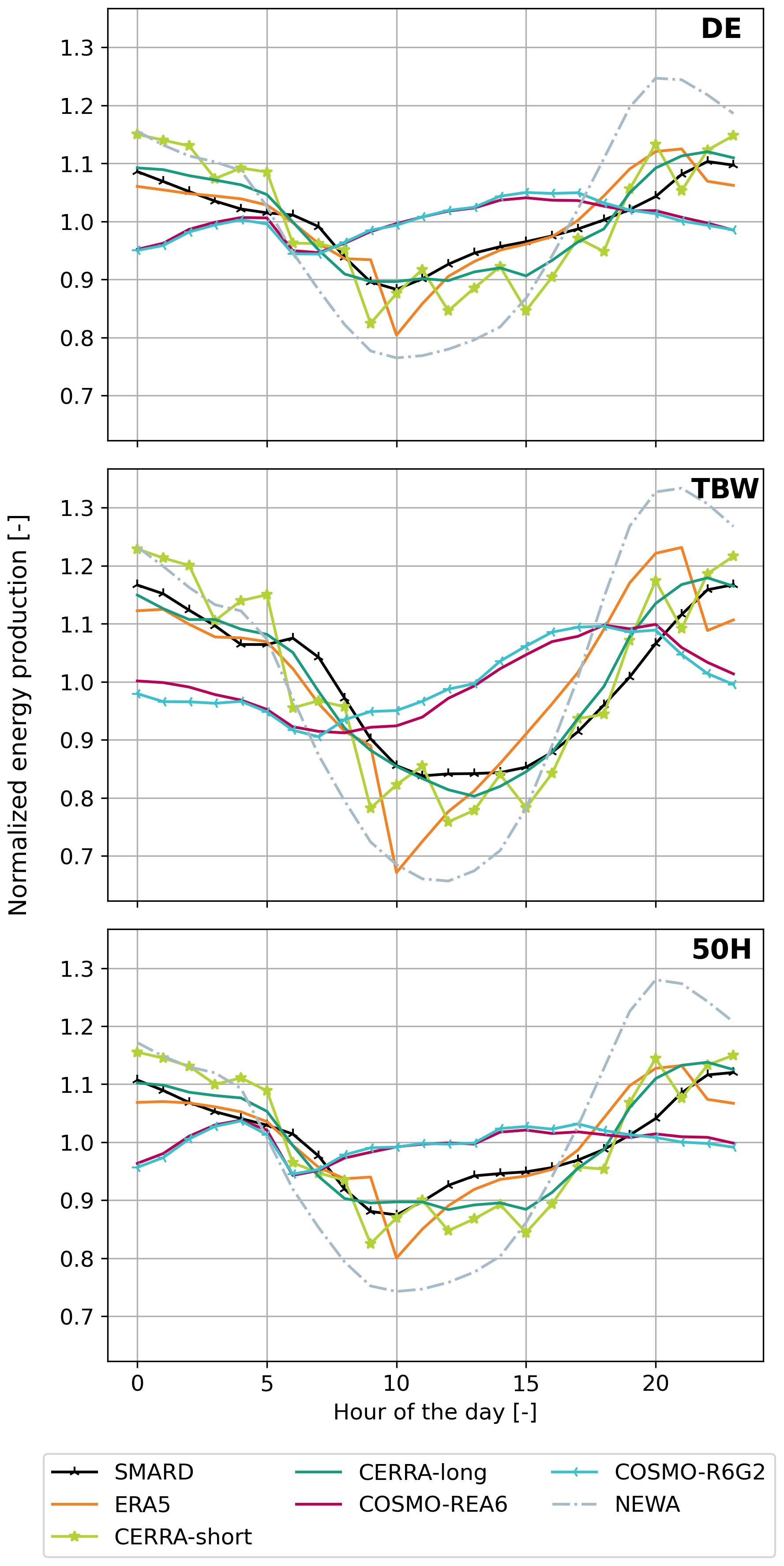
Figure 6 Normalised diurnal cycle of power production for Germany (DE), the TransnetBW control area (TBW) and the 50 Hz control area (50 Hz) in 2018. Shown are the SMARD data and the simulations based on ERA5, CERRA-long, CERRA-short, NEWA, COSMO-REA6 and COSMO-R6G2 in UTC.

Figure 6 illustrates the normalized diurnal cycle of power production for Germany (DE), the TransnetBW control area (TBW), and the 50 Hz control area (50 Hz) in 2018, comparing the SMARD data (black line) with the variouspower generation simulations. The power values are normalized to the average power generation.

The SMARD diurnal cycle exhibits a clear increase during nighttime, a decrease in the morning, and a gradual rise throughout the day for DE. All datasets, with the exception of COSMO-REA6 and COSMO-R6G2, display varying degrees of similarity to this pattern. The COSMO-based datasets deviate significantly from the measurements, probably due to problems with modelling the planetary boundary layer as described by Heppelmann et al. (2017). ERA5 shows a similar behaviour in the early hours compared to the SMARD cycle but experiences a sharp decline at 10:00 UTC. Jourdier (2020) initially reported the drop off as an issue and the ECMWF wiki acknowledges this behaviour but does not specify a reason (ECMWF, 2025). It states that the issue occurs at the change over from one assimilation cycle to the next, so it might be related to the assimilation pipeline. Following this drop, ERA5's power production increases at a comparable rate to SMARD, ultimately surpassing it around 16:00 UTC due to a faster rate of increase. A secondary, less pronounced drop at 22:00 UTC (also described by Jourdier (2020)) is observed in ERA5, suggesting that its performance may be a result of overestimation and underestimation cancelling out rather than consistent accuracy.

CERRA-short exhibits a distinctly jagged pattern, likely a consequence of merging short forecast windows, with each drop corresponding to a new analysis step every 3 h. The model begins with higher power production at night but declines more significantly during the day, only to increase more rapidly in the later hours. Conversely, in CERRA-long no jagged pattern is visible. The general diurnal pattern of both, CERRA-short and CERRA-long, closely aligns with SMARD, although its daytime increase is initially a little bit slower, and a little bit steeper than SMARD later during the day around 19:00 UTC.

NEWA begins at elevated levels compared to SMARD, but then dips lower, and later increases more rapidly. Its overall shape is smooth and in contrast to ERA5 and CERRA-short no artifacts are visible. The diurnal cycle of NEWA has a significantly higher amplitude than SMARD and all other datasets. The notable smoothness as well as the shape of the diurnal cycle is also found by Jourdier (2020) when analysing the diurnal cycle of the capacity factor time series for France. Since NEWA does not assimilate data in the modelling domain, this might be an indication that the drops and jagged behaviour in ERA5 and CERRA are related to the data assimilation.

The diurnal cycles of COSMO-REA6 and COSMO-R6G2 are nearly identical, differing only slightly between 13:00 and 18:00 UTC, where COSMO-R6G2 shows marginally higher values. Both datasets start lower than the others at night, gradually increasing until 05:00 UTC, followed by a slight dip before reaching their peak at 15:00 UTC and declining thereafter. Overall, their patterns are anti-correlated with SMARD at night and also significantly differ during the day. While all other datasets reproduce the general pattern of the diurnal cycle, COSMO-REA6 and COSMO-R6G2 fail to capture the average diurnal variations. This behaviour was also described for wind speed and capacity factors in France by Jourdier (2020) and for wind speed profiles in Germany by Bär et al. (2026).

The middle panel (TBW) depicts the TransnetBW control area, where the diurnal patterns broadly align with the DE trends. However, all diurnal cycles are more pronounced. In the SMARD data the difference between the minimum during daytime and the maximum during nighttime significantly increases by approximately 33 % and now varies between 0.84 and 1.15. All datasets, except COSMO-REA6 and COSMO-R6G2, show a strong correlation with the SMARD diurnal cycle.

ERA5 again closely matches SMARD during the night and early morning, with a more pronounced drop at 10:00 UTC and a steeper subsequent increase. The distinct drop at 22:00 UTC is even more pronounced than during day time. CERRA-short also exhibits increased variability in its drops but generally follows the SMARD trend. CERRA-long demonstrates the best agreement and reproduces the increase in diurnal variation in large parts. Only small deviations are visible from around noon into the evening where it drops slightly below SMRAD at 12:00 UTC and shows higher values from 16:00 UTC onwards.

NEWA remains smooth and shows the greatest variation compared to DE, with the lowest values shifting from 10:00 to 12:00 UTC. This results in a more pronounced U-shape. Its evening increase is stronger, with the maximum shifting from 20:00 to 21:00 UTC. As a result, the diurnal variation of NEWA is increased for TBW compared to DE.

COSMO-REA6 and COSMO-R6G2 diverge further from SMARD, showing increased variability in the diurnal cycle for TBW and a decrease in wind speeds during the early hours of the day. As for DE, both datasets are not able to reproduce the diurnal pattern of the energy production in the SMARD data.

The patterns in the diurnal cycle for 50 Hz are very similar to DE for the SMARD data and all investigated datasets. Only nuanced variations are visible with e.g. a slightly less pronounced peak of COSMO-REA6 and COSMO-R6G2 in the afternoon hours.

In summary the datasets show varying abilities to capture the diurnal cycle. In general ERA5 and especially CERRA were able to nicely reproduce the diurnal cycle for DE but also the variations between the control zones. However, CERRA-short and ERA5 exhibited artificial spikes. While NEWA can reproduce the overall pattern of the diurnal variations, its diurnal cycle has a significantly higher magnitude than the observations. COSMO-REA6 and COSMO-R6G2 do not capture the patterns of the diurnal cycle of the SMARD data. While the underlying models capture the diurnal cycle on the basis of atmospheric physics, the observed diurnal cycle is likely to be biased by several time-of-day-dependent loss categories. For example, curtailments due to bats and noise emissions only occur during the night. These influences on the diurnal cycle can only be taken into account by applying time-dependent loss factors by using i.e. detailed modelling approaches.

4 Conclusions

This study assessed the performance of different freely available reanalysis and meso-scale model datasets for modelling onshore wind power production in Germany. It demonstrated strong variations between the datasets in reproducing the annual energy production but also capturing the diurnal cycle in power production.

Interestingly the dataset with the lowest spatial resolution showed the best agreement to the recorded annual energy production for Germany. This indicates that increased spatial resolution does not necessarily mitigate systematic biases present in the models. In contrast the results of the study suggest that the country-wide biases were significantly increased for all regional downscalings. For all datasets an individual calibration of the wind data or simulated power production is advisable.

Regional analysis of the control zones revealed, that the dataset with the closest match to the recorded energy production changed depending on the region. An important factor is likely to be the terrain complexity. In flat terrain, simulations tend to overestimate production. In complex terrain, most datasets showed a closer match. This highlights the need for regional calibration, as country-wide calibration in e.g. Germany overemphasises wind turbines in flat regions and can introduce significant regional biases. Especially, when simulating developments in the future energy system this is critical, as regional turbine placement might differ significantly from the current turbine portfolio. It is also central for regional assessments like local grid expansion plans. In this context simple linear corrections on power production could provide good first corrections for ERA5 and CERRA for the current wind farm portfolio. For the other datasets, especially for NEWA, this correction is likely to perform worse. Additionally, theses corrections are based on the current wind turbine portfolio and should not directly be transferred to future expansion scenarios.

In general, the comparison of wind power production should not directly be translated to the average or typical wind conditions observed in the respective grid cells. Wind turbines are often constructed in locally windy locations. Therefore, the average wind speeds of the reanalysis datasets can be expected to have a higher overestimation than the comparisons of the wind energy production would suggest. This is especially important for areas with complex orography such as the TBW control zone, where turbines are placed in exposed locations like ridges and hilltops. As a consequence for wind power modelling this means that in addition to the regional differences also the topographic characteristics of the simulated wind farm portfolio should be considered when performing calibrations of wind speed or power generation. Another aspect that is important to consider when modelling future wind turbine portfolios is that they are likely to differ in technology – i.e. in hub height. In this case calibrations of wind speed from reanalysis datasets with the current wind farm portfolio can be misleading as the wind conditions and, thus, biases in the datasets and their ability to capture i.e. the diurnal patterns can change significantly with height. Future work should therefore address this using a large number of high quality wind measurements or analysis of wind power generation on individual turbine or wind farm level.

Most of the datasets analysed showed high correlations with the recorded wind energy production. However, significant differences could be observed. CERRA and ERA5 were clearly better in capturing temporal variations. The investigated datasets also show varying performance in capturing the diurnal cycle. CERRA-long shows the best agreement with the observed diurnal cycle. ERA5 exhibits good general performance, but its artificial drops require correction. Likewise, CERRA-short matches the diurnal pattern but is characterised by strong jagged patterns.

We have shown that both ERA5 and CERRA perform very well, with CERRA being slightly better. Therefore, wherever possible, we recommend using CERRA-long for wind energy applications. It has shown the best overall performance, especially in terms of diurnal cycle. The only drawback is the need for correction of energy production. But this is true in all models to some degree. ERA5 also performed very well, but the dips in the diurnal cycle and the underestimation in complex terrain need to be addressed. ERA5 is a good candidate for analysing large energy systems at national level in Germany and using the current wind farm portfolio – even without correction. In all other cases CERRA-long with regional bias correction seems to be preferable.

This study shows that the existing datasets are very useful and provide major benefits for energy systems analysis and wind resource assessment. Especially the high correlations on the national scale underline ERA5's and CERRA's capabilities to capture temporal patterns. However, the results also highlight several shortcomings – especially in systematic biases which vary with region and likely terrain characteristics. Therefore, further research into the physical parametrisations of the underlying atmospheric models as well as their temporal characteristics could yield significant additional benefits for wind energy applications.

Appendix A: Annual energy production

This section contains Fig. A1 showing the differences in annual energy production between the SMARD data and all investigated datasets in all investigated regions for 2017.

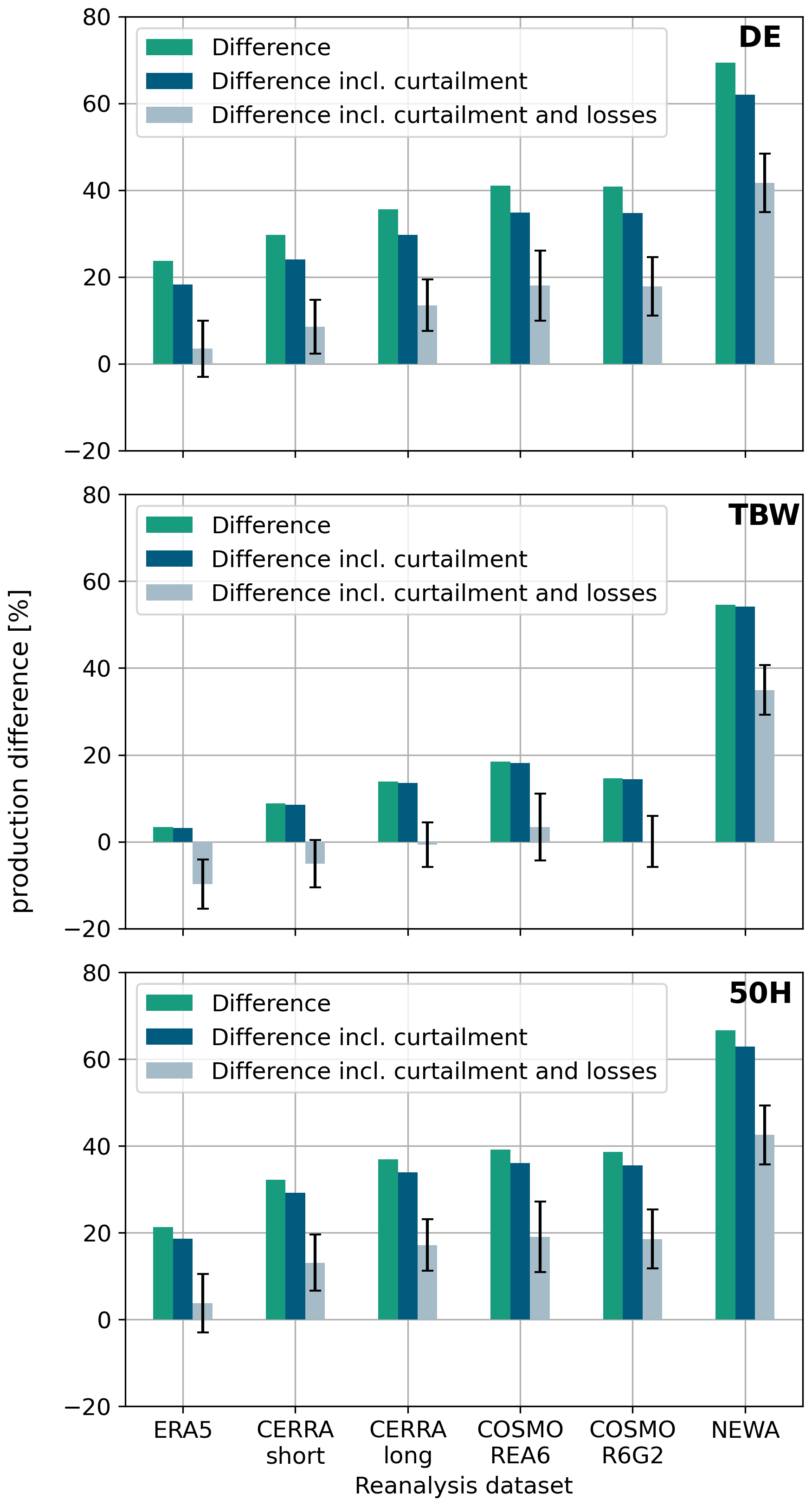
Figure A1 Differences in annual wind energy production between the SMARD data and different reanalysis datasets for Germany (DE), the TransnetBW control area (TBW), and the 50 Hz control area (50 Hz) in 2017. Differences are shown for raw production (green), accounting only for curtailment due to redispatch (blue) and accounting for curtailment due to redispatch and losses (grey). The black whiskers indicate a variation of ∓5 % in the estimated losses.

Appendix B: Correlation analysis

This section contains Fig. B1 showing the production scatter plots for CERRA-long, CERRA-short and COSMO-REA6 for 2018.

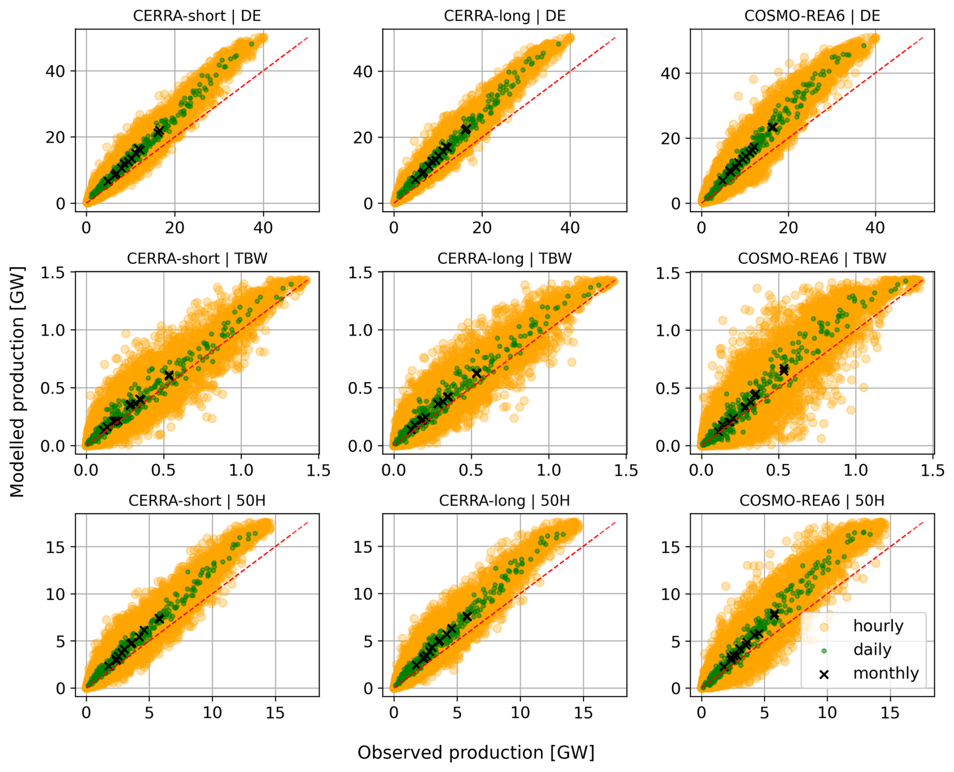
Figure B1 Scatter plots comparing simulated and observed hourly, daily and monthly energy production for 2018 for CERRA-long, CERRA-short and COSMO-REA6 for Germany (DE) and the investigated grid zones (TBW, 50 Hz). The dashed red line indicates the 1:1-line.