A possibilistic interpretation of ensemble forecasts: experiments on the imperfect Lorenz 96 system

Ensemble forecasting has gained popularity in the field of numerical medium-range weather prediction as a means of handling the limitations inherent to predicting the behaviour of high dimensional, nonlinear systems, that have high sensitivity to initial conditions. Through small strategical perturbations of the initial conditions, and in some cases, stochastic parameterization schemes of the atmosphere-ocean dynamical equations, ensemble forecasting allows one to sample possible future scenarii in a Monte-Carlo like approximation. Results are generally interpreted in a probabilistic way by building a predictive density function from the ensemble of weather forecasts. However, such a probabilistic interpretation is regularly criticized for not being reliable, because of the chaotic nature of the dynamics of the atmospheric system as well as the fact that the ensembles of forecasts are not, in reality, produced in a probabilistic manner. To address these limitations, we propose a novel approach: a possibilistic interpretation of ensemble predictions, taking inspiration from fuzzy and possibility theories. Our approach is tested on an imperfect version of the Lorenz 96 model and results are compared against those given by a standard probabilistic ensemble dressing. The possibilistic framework reproduces (ROC curve, resolution) or improves (ignorance, sharpness, reliability) the performance metrics of a standard univariate probabilistic framework. This work provides a first step to answer the question whether probability distributions are the right tool to interpret ensembles predictions.

1 Introduction

As a result of its chaotic dynamics, the prediction of the atmospheric system is particularly sensitive to the limited resolution in the initial conditions (ICs), discrepancies introduced by measurement error, computational truncation and an incomplete description of the system's dynamics (closure problem). Ensemble prediction systems (EPS) have consequently been developed to characterize the skill of single numerical predictions of the future state of the atmosphere. As suggested by Leith (1974), assuming that the error field is dominated by observational error (i.e. error on the ICs propagated forward in the model), we can perturb M times the best estimate for the ICs, run forward the model from each IC and interpret the M results in a Monte-Carlo like fashion. In other words, we use the local density of the resulting M predictions (or members) to quantify the plausibility of a given future scenario. Instead of the traditional point deterministic predictions, probabilistic predictions are thus realized. Today, the ICs are perturbed according to various schemes, designed to sample in a minimalist way systems of millions of dimensions (like numerical weather global models). These schemes generally select the initial perturbations leading to the fastest growing perturbations (e.g. singular vectors Hartmann et al., 1995).

Yet, in practice, the assumption of a near-perfect model, where observational error is more significant than model error, is not always true. Thus, individual member trajectories are not expected to stay in the convex hull of the ensemble after a few hours (Toth and Kalnay, 1997; Orrell, 2005). While ensemble predictions is built on the idea that the range of the ensemble provides an idea of the the possible futures and that its variance is representative of the skill of the single deterministic forecast, in practice and despite the introduction of stochastic parameterization schemes to represent model error (Buizza et al., 1999), the operational ensembles are overconfident: the spread is typically too small (Wilks and Hamill, 1995; Buizza, 2018). In particular, such probabilistic predictions are not reliable; on average, the probability derived for a given event does not equal the frequency of observation (Bröcker and Smith, 2007; Smith, 2016; Hamill and Scheuerer, 2018). Although ensemble-based probabilistic predictions present more skill than the climatology, they generally cannot be used as actionable probabilities. By design (limited EPS size, biased sampling of ICs) and by context (flow-dependent regime error, strongly nonlinear system) they do not represent the true probabilities of the system at hand (Legg and Mylne, 2004; Orrell, 2005; Bröcker and Smith, 2008). This is all the more true for extreme events, that, for dynamical reasons, cannot be associated to a high density of ensemble members; such events indeed result from nonlinear interactions at small scales, which cannot be reproduced in number in a limited-size EPS (Legg and Mylne, 2004).

A range of post-processing methods have been developed to tackle these limitations (Vannitsem et al., 2018). The classical Bayesian model averaging (BMA; Raftery et al., 2005) and non-homogeneous Gaussian regression (Gneiting et al., 2005) fit an optimized (sum of) parametric distribution(s) onto the ensemble of predictions. More recently, techniques involving recalibration by means of the probability integral transform (Graziani et al., 2019) or by using the actual probability of success of a given probabilistic threshold (Smith, 2016) were particularly designed to address the lack of reliability of the previous approaches. Similarly, (Hamill and Scheuerer, 2018) improved notably the reliability of probabilistic precipitation forecasts by means of quantile mapping and rank-weighted best-member dressing over single or multimodel EPS. Changing perspective, Allen et al. (2019) introduced a regime-dependent adaptation of the traditional post-processing parametric methods, to tackle the issue of possibly significant model error. All ensemble post-processing techniques are trained on an archive set of (ensemble, observation) pairs, using the same model. Most often, the objective function to optimize is a performance score, like the negative log-likelihood or the continuous ranked probability score, whose individual results for each couple (ensemble, verification) are aggregated over the whole archive.

However, if generic strategies for post-processing globally improves the skill for common events, they tend to deteriorate the results for extreme events (Mylne et al., 2002). The latter are indeed, for predictability reasons, less susceptible to be associated to a high density of ensemble members (Legg and Mylne, 2004).

For all these reasons, and especially the need to resort to multiple post-processing steps to provide meaningful probabilistic outputs, we may wonder, echoing Bröcker and Smith (2008), whether the probability distribution (PDF) is the best representation of the valuable information contained in an EPS. Rather, the description of possibility theory in Dubois et al. (2004): “a weaker theory than probability (…) also relevant in non-probabilistic settings where additivity no longer makes sense and not only as a weak substitute for additive uncertainty measures” presents new opportunities, in a context where conceptual and practical limitations restrict the applicability of a density-based (i.e. additive) interpretation of EPS.

This is what we investigate in this work. Namely: can we design a simple possibilistic framework for interpreting EPS that would perform at least as well as a standard probabilistic approach for most of the performance metrics, and improve the known shortcomings of the probabilistic approach? We investigate this question by means of numerical experiments on a commonly-used surrogate model of the atmospheric dynamics, the Lorenz 96 system. Section 2 introduces the basics of possibility theory, then used to develop an original possibilistic framework for the interpretation of ensemble of predictions in Sect. 3. This framework is tested on the imperfect Lorenz 96 model in Sect. 4. A conclusion follows.

2 Possibility theory

Possibility theory is an uncertainty theory developed by Zadeh (1978) from fuzzy set theory. It is designed to handle incomplete information and represent ignorance. Considering a system whose state is described by a variable x∈𝒳, the possibility distribution $\mathit{\pi }:\mathcal{X}\mapsto [\mathrm{0},\mathrm{1}]$ represents the state of knowledge of an agent about the current state of the system. Given an event $A=\mathit{\{}x\in S_A\mathit{\}}$, the possibility and necessity measures are defined respectively as: $\mathrm{\Pi }\left(A\right)={sup}_{x\in S_A}\mathit{\pi }\left(x\right)$ and $N\left(A\right)=\mathrm{1}-\mathrm{\Pi }\left(\stackrel{\mathrm{‾}}{A}\right)$ where $\stackrel{\mathrm{‾}}{A}$ represents the complementary event of A. Π(A) and N(A) satisfy the following axioms:

1. Π(𝒳)=1 and Π(∅)=0

2. $\mathrm{\Pi }(A\cup B)=max\left(\mathrm{\Pi }\right(A),\mathrm{\Pi }(B\left)\right)$ (similar to $N(A\cap B)=min\left(N\right(A),N(B\left)\right)$), where $B=\mathit{\{}x\in S_B\mathit{\}}$.

The following conventions apply (Cayrac et al., 1994):

• a.

  $N\left(A\right)=\mathrm{1}\iff \mathrm{\Pi }\left(\stackrel{\mathrm{‾}}{A}\right)=\mathrm{0}$ indicates that A has to happen, it is necessary;

• b.

  $\mathrm{0}<N\left(A\right)<\mathrm{1}$ is a tentative acceptance of A to a degree N(A), since $min\left(N\right(A),N(\stackrel{\mathrm{‾}}{A}\left)\right)=\mathrm{0}$ from axiom 2 ($\stackrel{\mathrm{‾}}{A}$ is not necessary at all);

• c.

  $\left(\mathrm{\Pi }\right(A)=\mathrm{\Pi }(\stackrel{\mathrm{‾}}{A})=\mathrm{1})\iff \left(N\right(A)=N(\stackrel{\mathrm{‾}}{A})=\mathrm{0})$ represents total ignorance: the evidence doesn't allow us to conclude if A is rather true or false;

Possibility and probability distributions are interconnected, through the description of uncertainty by imprecise probabilities (cf. the Dempster-Shafer Theory of Evidence's framework; Dempster, 2008). Under specific constraints, an imprecise distribution can degenerate into either a probability or a possibility distribution. One can consequently assess the degree of consistency of a possibility and a probabilistic distributions. Among the definitions of consistency (Delgado and Moral, 1987), we retain here the view of Dubois et al. (2004), that a probability measure P and possibility measure Π are consistent if the probability of all possible events A satisfies P(A)≤Π(A). It implies, from the definition of necessity, that the probability P(A) is bounded as well from below by the necessity measure: $N\left(A\right)\le P\left(A\right)\le \mathrm{\Pi }\left(A\right)$. Necessity and possibility measures can consequently be viewed as upper and lower limits on the probability of a given event.

3 Possibilistic framework for EPS interpretation

The statistical post-processing of EPS generates forecasts in the form of predictive probability distributions $p\left(x\right|\stackrel{\mathrm{̃}}{\mathit{x}},\mathit{\theta })$, noted $p\left(x\right|\stackrel{\mathrm{̃}}{\mathit{x}}{)}_{\mathit{\theta }}$, where $\stackrel{\mathrm{̃}}{\mathit{x}}=\mathit{\{}{\stackrel{\mathrm{̃}}{x}}_{\mathrm{1}},\mathrm{\dots },{\stackrel{\mathrm{̃}}{x}}_M\mathit{\}}$ is the ensemble, θ a vector of parameters and p a (sum of) parametric distribution(s). BMA distributions are weighted sums of M parametric probability distributions, each one centered around a linearly corrected ensemble member. In this work, the members are exchangeable, so the mixture coefficients and parametric distributions do not vary between members and the BMA comes down to an ensemble dressing procedure. We compare our method against a Gaussian ensemble dressing, whose predictive probability distribution reads:

$$\begin{array}{}\text{(1)}& p\left(x\right|\stackrel{\mathrm{̃}}{\mathit{x}}{)}_{\mathit{\theta }}={\displaystyle \frac{\mathrm{1}}{M}}\sum _{i=\mathrm{1}}^M\mathcal{N}(a{\stackrel{\mathrm{̃}}{x}}_i+\mathit{\omega },{\mathit{\sigma }}^{\mathrm{2}})\end{array}$$

where 𝒩(μ,v) is the normal distribution of mean μ and variance v. The parameters $\mathit{\theta }=\mathit{\{}a,\mathit{\omega },\mathit{\sigma }\mathit{\}}$ are inferred through the optimization of a performance metric, e.g. the ignorance score (Roulston and Smith, 2002), or negative log-likelihood, a strictly proper¹ and local² logarithmic score.

Here, instead of performing a probabilistic ensemble dressing, we can perform a possibilistic ensemble dressing: a possibilistic membership function is dressed around each ensemble member first shifted and scaled. Similarly to its probabilistic twin, the ith possibility kernel is assumed to represent the possibility distribution of the true state of the system, given the observation of ${\stackrel{\mathrm{̃}}{x}}_i$. Because we have several member observations $i=\mathit{\{}\mathrm{1},\mathrm{\dots },M\mathit{\}}$ and there is only one truth (the actual system's state), we can interpret it as a union (OR) of possibilities. Fuzzy set theory offers several definitions for computing the distribution resulting of the union of two fuzzy distributions. We adopt here the max-sum definition: ${\mathit{\pi }}_{A\cup B}\left(x\right)=max\left({\mathit{\pi }}_A\right(x),{\mathit{\pi }}_B(x\left)\right)$, although some of our tests, not presented here, show that alternative definitions do not significantly change results.

Gaussian kernels ${\exp }^{-\frac{\mathrm{1}}{\mathrm{2}}{u}_i^{\mathrm{2}}}$ are thus fitted to each member ${\stackrel{\mathrm{̃}}{x}}_i$, with $u_i=\frac{x-(a{\stackrel{\mathrm{̃}}{x}}_i+\mathit{\omega })}{\mathit{\sigma }}$, a the scaling factor, ω the shifting of the kernels' peaks from the individual member ${\stackrel{\mathrm{̃}}{x}}_i$ and σ a parameter accounting for the width of the individual kernels. The resulting possibilistic distribution is given by the sum, in a possibilistic manner, of all the individual kernels:

$$\begin{array}{}\text{(2)}& \begin{array}{rl}\mathit{\pi }\left(x\right)& ={\cup }_{i=\mathrm{1}\mathrm{\dots }M}{\exp }^{-\frac{(x-(a{\stackrel{\mathrm{̃}}{x}}_i+\mathit{\omega }){)}^{\mathrm{2}}}{\mathrm{2}{\mathit{\sigma }}^{\mathrm{2}}}}\\ & =\underset{i=\mathrm{1}\mathrm{\dots }M}{sup}{\exp }^{-\frac{(x-(a{\stackrel{\mathrm{̃}}{x}}_i+\mathit{\omega }){)}^{\mathrm{2}}}{\mathrm{2}{\mathit{\sigma }}^{\mathrm{2}}}}\end{array}\end{array}$$

For any event of interest $A=\mathit{\{}x\in S_A\mathit{\}}$, we can extract the possibility and necessity measures Π(A,θ) and N(A,θ) (noted Π_θ(A) and N_θ(A)), given the knowledge encoded in π(x,θ) (noted π_θ). Π_θ(A) evaluates to what extent A is logically consistent with π_θ whereas N_θ(A) evaluates to what extent A is certainly implied by π_θ. Ideally, this pair falls in an area of the possibilistic diagram (N,Π) that is close to one of the three notable points: (1,1) for A certain; (0,0) for $\stackrel{\mathrm{‾}}{A}$ certain; (0,1) for total ignorance, i.e. both A and $\stackrel{\mathrm{‾}}{A}$ are possible but none is necessary given π. Points on the line N=0 are in favor of $\stackrel{\mathrm{‾}}{A}$, the more favorable the closer to (0,0); points on the line Π=1 are in favor of A, the more favorable the closer to (1,1). Other areas of the diagram are inconsistent with the axioms defining Π and N.

From the geometric interpretation given by the possibilistic diagram, several options are available for scoring each point (N_θ(A),Π_θ(A)) that is, for assessing the quality of the prediction given by the pair (N_θ(A),Π_θ(A)).

A brute-force method is to minimize the distance to the correct pole (e.g. (1,1) for A true). Yet, such an approach would try and push events towards (1,1) or (0,0) on the possibilistic diagram, thus ignoring the ignorance pole and, as a result, the idea that some events are impossible to predict from a particular EPS set. A more complete method could, for instance, also consider the rank r of the EPS w.r.t. A. Namely, if the actual observation x^* is in S_A, the associated point should belong to the line Π=1 but the distance to the ignorance pole (1,0) should be proportional to r. The same applies for $x^{*}\notin S_A$; the associated point should belong to line N=0 with the distance to (1,0) proportional to $r_{\stackrel{\mathrm{‾}}{A}}=M-r_A$. Thus, an observation $x^{*}\in S_A$ associated to an erroneous EPS (r→0) will fall close to the ignorance pole, suggesting that we cannot trust the raw ensemble. A score verifying these requirements is:

$$S_i\left(\mathit{\theta }\right)=\left\{\begin{array}{l}\left|N_{\mathit{\theta }}\right(A)-\frac{r}{M}|+\left|{\mathrm{\Pi }}_{\mathit{\theta }}\right(A)-\mathrm{1}|,x^{*}\in S_A\\ N_{\mathit{\theta }}\left(A\right)+\left|{\mathrm{\Pi }}_{\mathit{\theta }}\right(A)-\frac{r}{M}|,x^{*}\notin S_A\end{array}\right.$$

Given a training set containing n pairs $({\stackrel{\mathrm{̃}}{\mathit{x}}}_i,x_i^{*})$, the final empirical score is: $S\left(\mathit{\theta }\right)=\frac{\mathrm{1}}{n}{\sum }_{i=\mathrm{1}}^n{S}_i\left(\mathit{\theta }\right)$ and training consists of finding the θ that minimizes S.

4 Application to the imperfect Lorenz 96 system

To test our framework, we reproduce the experiment designed by Williams et al. (2014), who used an imperfect L96 model (Lorenz, 1996) to generate ensemble predictions and investigate the performance of ensemble post-processing methods for the prediction of extreme events. The training sets consist of 4000 independent pairs of EPS of size M=12 and the associated observations, for each lead time $\mathit{\tau }=\mathit{\{}\mathrm{1},\mathrm{3},\mathrm{5},\mathrm{7}\mathit{\}}$ d³. The EPS have beforehand been pre-processed to remove the constant bias. The testing set consists of another 10 000 independent pairs of bias-corrected EPS and associated observations, for each lead time. We consider the prediction of an extreme event: $A_{\mathrm{e}}=\mathit{\{}x\le q_{\mathrm{0.05}}\mathit{\}}$, where q_0.05 is the quantile 5 of the climatic distribution of x and a common event $A_{\mathrm{c}}=\mathit{\{}{q}_{\mathrm{0.5}}\le x\le q_{\mathrm{0.6}}\mathit{\}}$ . Results are compared against those given by a probabilistic post-processing, namely a Gaussian ensemble dressing.

We first assess the performance of each interpretation in terms of the empirical ignorance score relative to the climatology:

$$\begin{array}{}\text{(3)}& \begin{array}{rl}{S}_n(p_{\mathit{\theta }},c)& ={\displaystyle \frac{\mathrm{1}}{n}}\sum _{i=\mathrm{1}}^n\left(\mathrm{IGN}\right(r_{\mathit{\theta }},x_i^{*})-\mathrm{IGN}(c,x_i^{*}\left)\right)\\ & =-{\displaystyle \frac{\mathrm{1}}{n}}\sum _{i=\mathrm{1}}^n{\log }_{\mathrm{2}}\left({\displaystyle \frac{r_{\mathit{\theta }}\left(x_i^{*}\right)}{c\left(x_i^{*}\right)}}\right)\end{array}\end{array}$$

where, following the work of Bröcker and Smith (2008), in the probabilistic framework, the predictive probability $p_{\mathit{\theta }}\left(x^{*}\right|\stackrel{\mathrm{̃}}{\mathit{x}})$ is blended with the climatology c(x^*) of the verification x^*: $r_{\mathit{\theta }}\left(x^{*}\right)=\mathit{\alpha }{p}_{\mathit{\theta }}\left(x^{*}\right)+(\mathrm{1}-\mathit{\alpha })c\left(x^{*}\right)$. Our possibilistic framework is a mapping ${\mathbb{R}}^M\mapsto [\mathrm{0},\mathrm{1}]\times [\mathrm{0},\mathrm{1}]$, while the ignorance applies to a probabilistic prediction ${\mathbb{R}}^M\mapsto [\mathrm{0},\mathrm{1}]$. We consequently need to find a mapping from the dual measures N and Π to an equivalent probability. Since possibility and necessity measures can be seen as upper and lower bounds of a consistent probability measure, we can write $P_{\mathit{\alpha }}\left(A\right)=\mathit{\alpha }N\left(A\right)+(\mathrm{1}-\mathit{\alpha })\mathrm{\Pi }\left(A\right)$ with $\mathit{\alpha }\in [\mathrm{0},\mathrm{1}]$ for any event A of interest. Varying α allows one to browse across the range of associated probabilities P(A), consistent with the possibility distribution π. We use this technique to compute the ignorance score of the possibilistic framework and compare its range to the performance of a probabilistic Gaussian ensemble dressing.

Both frameworks are characterized by negative relative ignorance, confirming that they have a predictive added-value over climatology. The difference in ignorance equals the difference in expected returns that one would get by placing bets proportional to their probabilistic forecasts.

As shown in Fig. 1, for both types of events, the possibilistic framework performs as well or slightly better than the probabilistic, for all $\mathit{\alpha }\in [\mathrm{0},\mathrm{1}]$. The slight increase in performance remains relatively constant or even improve (extreme event case) with lead time. The relative ignorance of the possibilistic framework has a variance (due to the range of α) that grows with the lead time, as expected.

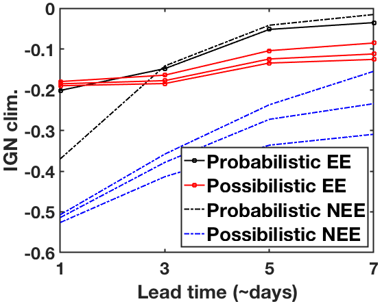
Figure 1 Ignorance relative to the climatology computed for the possibilistic (colored lines) and probabilistic (black lines) frameworks, in the case of the prediction of an extreme (EE; solid line) and a common (NEE; dashed line) event of interest, as defined in Sect. 4. The upper and lower bounds, as well as the median, obtained by considering that $N\left(A\right)\le P\left(A\right)\le \mathrm{\Pi }\left(A\right)$ in the possibilistic framework are reported.

To understand better the operational consequences of such results, we report in Fig. 2 the relative operating characteristic (ROC) of both frameworks at lead times of 3 and 7 d. Given a binary prediction (yes/no w.r.t. event A), the ROC plots the hit rate (HR; fraction of correctly predicted A over all A observed) versus the false alarm rate (FA; fraction of wrongly predicted A over all $\stackrel{\mathrm{‾}}{A}$ observed). We use increasing thresholds $p_t\in [\mathrm{0},\mathrm{1}]$ for making the decision (yes if P(A)≥p_t) and report the associated HR and FA in the graph. Again, we vary α to see the range of HR and FA covered for each p_t by the possibilistic prediction (N,Π). The resulting points form a curve (probabilistic approach) or a cloud (possibilistic method), which are a visual way to assess the ability of a forecast system to discriminate between events and non events.

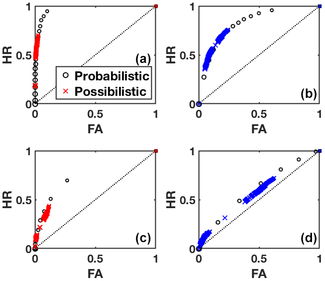
Figure 2 ROC curves for the extreme event (a, c) and common event (b, d) at lead time 3 d (a, b) and 7 d (c, d). The probabilistic results are reported by means of black circles and the possibilistic results by means of colored crosses. The larger the symbol, the larger the threshold probability used to compute HR and FA.

The possibilistic curves all fit or are very close to the probabilistic curves, for both extreme and common events and for all lead times. The main difference is their extension: the possibilistic framework remains located in areas of relatively small FA, compared to the results of the probabilistic approach for similar thresholds p_t. This results indicates that the HR remains smaller than what can be achieved by the probabilistic framework, showing lower skill. The fact that the possibilistic curves yet lies on the probabilistic ROC curves shows that the reason behind this discrepancy is not a lack of discrimination between events and non-events; for a given FA, both methods provide the same HR. The reason is connected to a bias in probabilities for the possibilistic approach towards zero and towards 1: the possibilistic framework is very sharp, as shown on the diagrams in Fig. 3. Because they are not blended with climatology, a large part of the predictions have zero probability associated to the event of interest, instead of a minimal one, which prevents the current implementation of the possibilistic framework from reaching higher HR. Side experimentation not reproduced here has shown that weighting the scores attributed to observed event A in the global empirical training score allows to reproduce fully the probabilistic curve for each lead time.

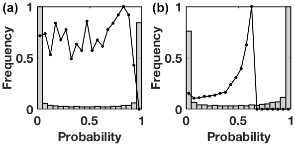
Figure 3 Normalized histograms of the equivalent forecast probabilities in the possibilistic framework for the observations of the extreme event (a) and common event (b) at lead time 3 d. The corresponding distributions of predictive probabilities in the probabilistic framework come on top as thick black lines.

Reliability diagrams presented on Fig. 4 plot the observed conditional frequencies against the corresponding forecast probabilities for lead time 3 and 7 d. They illustrate how well the predicted probabilities of an event correspond to their observed conditional frequencies. The predictive model is all the more reliable (i.e. actionable) when the associated curve is close to the diagonal. Noting that the diagonal represents perfect reliability, the distance to the diagonal indicates underforecasting (curves above) or overforecasting (curves below). Distance above the horizontal climatology line indicates a system with resolution, a system that does discriminate between events and non-events. The cones defined by the no-skill line (half-way between the climatology and perfect reliability) and the vertical climatology line allow us to define areas where the forecast system is skilled.

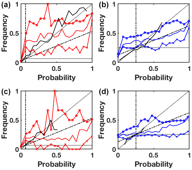
Figure 4 Reliability diagrams for the extreme event (a, c) and common event (b, d) at lead time 3 (a, b) and 7 d (c, d). The probabilistic results are reported in black line, while the upper, median and lower bounds of the possibilistic ones are in thinner red lines. Standards elements of comparison are reported in the diagram, as described in Sect. 4, namely the diagonal (perfect reliability), the climatological reference (horizontal dotted) and the cones of skill (inside the dashed-dotted secants).

To draw a standard reliability diagram from possibilistic predictions, we use again the transformation: $P_{\mathit{\alpha }}\left(A\right)=\mathit{\alpha }N\left(A\right)+(\mathrm{1}-\mathit{\alpha })\mathrm{\Pi }\left(A\right)$, where α is discretized on [0,1]. From a given set of n predictions (N(A),Π(A)), for each ${\mathit{\alpha }}_i\in [\mathrm{0},\mathrm{1}]$, the n $P_{{\mathit{\alpha }}_i}\left(A\right)$ are computed and a traditional reliability plot is drawn. Each α_i-plot indicates how using $P_{{\mathit{\alpha }}_i}\left(A\right)$ as probability for A is reliable and actionable on the long term. The upper and lower bounds on the set of corresponding plots correspond respectively to the cases P_α(A)=N(A) and P_α(A)=Π(A). Seen as a whole, this bounded set of reliability plots allows to characterize the reliability of the probabilities given through the relation $N\left(A\right)\le P\left(A\right)\le \mathrm{\Pi }\left(A\right)$.

As pictured on Fig. 4, probabilistic curves are globally aligned with the perfect reliability line, yet with growing lead time, they are restricted to small probabilities only (because of wider EPS or pure predictability issues such as mentioned for extreme events). On the contrary, the reliability plots associated with the possibilistic approach cover all range of probabilities. This approach tends to be underforecasting (resp. overforecasting) for small (resp. large) probabilities, especially for the common event. A large part of the area covered by the possibilistic solutions is contained in the skill cones for the rare event, denoting a skilled predictive system for all but very low predictive probabilities. Results are less interesting for the common event, where the possibilistic framework leads to a flatter diagram, indicating less resolution, especially with larger lead times.

Such a 2-dimensional fuzzy reliability diagram is neither particularly operational nor easy to read. To adapt it to the specificity of our dual predictive measures, we suggest to use 3-dimensional reliability-like diagrams. We consider the two axes of the N−Π diagram potentially occupied by prediction points: N=0 and Π=1, other areas being inconsistent with axiom (b) from Sect. 2. Each axis is binned and the frequency of observation of the event A among the prediction points that fall in each bin is computed. Results are plotted on a third vertical axis, added to the N−Π diagram. It allows to assess quickly and visually the distribution of the successful predictions for event A over the diagram, by associating to each bin a frequency of success. A good behaviour would be to observe a decreasing frequency along both axis from (1,1) to (0,0): the closer to the points of certainty (N(A)=1 and $N\left(\stackrel{\mathrm{‾}}{A}\right)=\mathrm{1}-\mathrm{\Pi }\left(A\right)=\mathrm{1}$ respectively), the maximal the probability of observing A (resp. $\stackrel{\mathrm{‾}}{A})$. There is no constraint on the ignorance point: over all the points that did not provide enough information to decide, there is no reason that the frequency of observation of A is 0.5. It could be the climatological frequency c(A), if the lack of information is randomly distributed among observations. The fact that the frequency of observation of A at the ignorance point is actually larger than c(A) may be an indication of model limitations for the prediction of this type of event, e.g. due to particular dynamics that fail to be captured: they systematically, more often than not, lead to undecidability based on the information at hand. Figure 5 presents such 3-dimensional reliability diagrams for lead times 1 and 7 d. As suggested before, the framework tends to show lower discrimination for the prediction of the common event: predictions on the Π=1 axis guarantee a high level of success for the extreme event, while this level decreases quickly with smaller N for the common event.

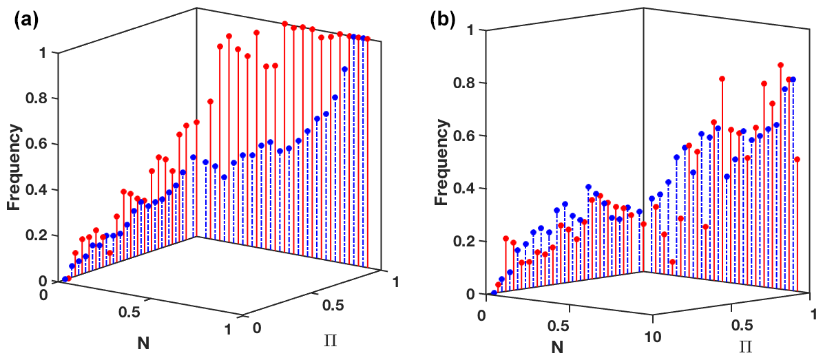
Figure 5 3-dimensional reliability diagrams for the extreme event (solid red lines) and common event (dashed blue lines) at lead time 1 (a) and 7 d (b). They assess the frequency of observation of the event A when the possibilistic prediction (N(A),Π(A)) falls in a given bin on the N−Π diagram.

5 Conclusions

In this work, we have presented a possibilistic framework which allows us to interpret ensemble predictions without the notion of member density, or additivity that proved to be incoherent with the conditions in which EPS were built. Preliminary results show that such a framework can be used to reproduce the probabilistic performances (ROC curves, resolution) and even slightly improve some of them (ignorance, sharpness, reliability). The added-value of this framework is more tangible for extreme events. Moreover, the proposed approach addresses some of the well-known limitations of the probabilistic framework (reliability, for example), in a simpler setting than the multiple post-processing steps usually necessary to address these limitations (e.g. (Hamill and Scheuerer, 2018; Graziani et al., 2019). We can consequently indeed wonder whether a framework based on imprecise probabilities, like possibility theory or credal sets of distributions (echoing Berger and Smith, 2019) is not indeed more appropriate to make sense and extract in a simpler manner the valuable information contained in an EPS.

We have introduced as well a first tool, namely the 3-dimensional reliability diagram, to make operational sense of the dual possibilistic predictions. However, further work is needed to improve the design of the possibilistic distributions, by means for instance of dynamical information.

Finally, since our predictive model is based on the optimization of a set of parameters (shaping possibilistic kernels on EPS members), it involves a trade-off on the performance of each individual case in the training set. The authors will address this question by means of a new framework free of parameters and consequently free of optimization. Such a framework will allow the measures (N,Π) to be guaranteed formally (which the current optimization step does not allow) and to provide meaningful values for each individual prediction.

Developments regarding the understanding and the operational use of such fuzzy results are necessary and will be developed as well in the future work mentioned above.