Evaluation of ERA5, MERRA-2, COSMO-REA6, NEWA and AROME to simulate wind power production over France

As variable renewable energies are developing, their impacts on the electric system are growing. To anticipate these impacts, prospective studies may use wind power production simulations in the form of 1 h or 30 min time series that are often based on reanalysis wind-speed data. The purpose of this study is to assess how several wind-speed datasets are performing when used to simulate wind-power production at the local scale, when no observation is available to use bias correction methods. The study evaluates two global reanalysis (MERRA-2 from NASA and ERA5 from ECMWF), two high-resolution models (COSMO-REA6 reanalysis from DWD, AROME NWP model from Météo-France) and the New European Wind Atlas mesoscale data. The study is conducted over continental France. In a first part, wind-speed measurements (between 55 and 100 m above ground) at eight locations are directly compared to modelled wind speeds. In a second part, 30 min wind-power productions are simulated for every wind farm in France and compared to two open datasets of observed production published by the distribution and transmission system operators, either at the local scale in terms of annual bias, or aggregated at the regional scale, in terms of bias, correlations and diurnal cycles. ERA5 is very skilled, despite its low resolution compared to the regional models, but it underestimates wind speeds, especially in mountainous areas. AROME and COSMO-REA6 have better skills in complex areas and have generally low biases. MERRA-2 and NEWA have large biases and overestimate wind speeds especially at night. Several problems affecting diurnal cycles are detected in ERA5 and COSMO-REA6.

1 Introduction

In the past ten years, wind and photovoltaic powers have been steadily developing in France. Their installed capacities have risen above respectively 16 and 9 GW in 2019 (RTE, 2020a). The development shall continue as the country's goals of installed capacity by 2028 are about 40 GW for wind (including 6 GW offshore) and 35 to 44 GW for photovoltaic power (Ministère de la Transition écologique et solidaire, 2020).

As their shares increase in the electricity mix, so do their impacts on the electrical system. They have physical impacts on the distribution grid at the local scale and on the transmission network at larger scales. They also have financial impacts as they modify the prices on the electricity market (Paraschiv, 2014). They impact the other generation units through prices and also because they modify the residual load (demand minus variable renewable generation) left to the dispatchable power stations. Very high shares of variable renewable energy bring new challenges in terms of network development, flexibility needs, frequency stability or market design (Silva et al., 2018) and they increase the system sensitivity to climate variability (Bloomfield et al., 2016).

To conduct prospective studies assessing those various impacts, input data are usually simulations of the necessary parametres: wind-power generation (which will be the focus here) but also other energy generations, demand, etc. depending on the scope of the study. Recent years have seen the development of several simulation datasets, such as Ninja (Staffell and Pfenninger, 2016), EMHIRES (Gonzales-Aparicio et al., 2016), RE-Europe (Jensen and Pinson, 2017), the University of Reading (UR) dataset (Bloomfield et al., 2019) or the upcoming data from Copernicus Climate Change Service (C3S) for Energy, in the continuity of the C3S ECEM project (Troccoli et al., 2018). These datasets provide simulations at aggregated levels (regions or countries; grid nodes for RE-Europe). Only Ninja offers local simulations through the web interface https://www.renewables.ninja/ (last access: 10 May 2020). Some studies require local simulations, for example to investigate impacts on the distribution grid from a future wind farm or set of farms in a specific region. This study focuses on simulations used for local-scale applications.

Simulations are usually based on wind-speed data from climate reanalyses are they are useful data with large spatial and temporal coverage. For example, the above-mentioned datasets are based on global reanalyses: MERRA-2 (Ninja, EMHIRES), ERA-Interim (ECEM), ERA5 (UR, C3S Energy) or on COSMO-REA6 regional reanalysis for RE-Europe, which is simulating at a finer scale (grid nodes). Indeed, local simulations could benefit from using higher resolution models than the global reanalyses used for national-scale simulations. In this study, three high-resolution datasets are evaluated in addition to two global reanalyses.

Simulations use wind-power modelling techniques to convert wind-speed data into power output. Those conversion models are of two main types: statistical or physical. Statistical methods use observed production data to train a statistical (e.g. machine learning) model (example in ECEM). They require that the farm exists (thus not applicable in prospective studies) and that past production data are accessible (not confidential). On the other hand, physical methods use turbine power curve functions to convert hub-height wind speeds to power output. Physical methods are used in all the above-mentioned simulations (ECEM tests both methods). This approach requires at least basic information on the technology: the model or type of wind turbine to select an adequate power curve and the hub height to extrapolate wind-speed at this level. The main drawback of this approach is that biases in the underlying wind-speed data may create huge under or over-estimations of power outputs. This is why this approach is often combined with a bias correction model. For example in Ninja, observed national productions are compared to aggregated simulations to fit a wind-speed correction model in each country. Another example is the use of statistical downscaling of the global reanalysis using another higher-resolution dataset. For example EMHIRES and UR use data from the Global Wind Atlas to modify locally the distributions of the reanalysis data. But using another numerical dataset with its own biases is not necessary beneficial. The same downscaling technique shows no improvement in Gruber and Schmidt (2019). In this paper purely physical methods are investigated to be able to use them when no observation is available, neither wind-speed observation to unbias the input data, nor past production to train a statistical model. Statistical downscaling of reanalysis data are not studied here except in the sense that the high resolution models evaluated here might be used for bias corrections, if not used directly.

Other applications are also using wind-power modelling. Even thought they are not the topic of this study, they are worth mentioning as they share common data and methods. One field of applications is wind resource assessment prior to a farm installation (Brower, 2012). In early planning stages, numerical datasets are used in the form of wind atlases, which commonly provide summarized statistics about local wind speeds. In more mature phases, wind farm developers install masts or LIDAR to measure wind speeds at the project’s location. Applications where local wind-speed observations are available are not the scope of this study. Such measurements enable to either simulate directly from the observed wind speeds or to apply bias corrections thus significantly reducing the uncertainty about the on-site winds and the power simulations. Another field of applications is power forecasting from hourly (Giebel and Kariniotakis, 2017, for a review) to seasonal timescales (e.g. Lledó et al., 2019) based on operational numerical weather prediction (NWP) models. Forecasting is done for operational farms, so observed past production is usually available to train a statistical model or at least correct the biases of a physical model. Forecasts are not the scope of this study and will not be discussed here. Simulations however may be used in place of observations in order to train a statistical forecasting system, for example for a new wind farm that has no or not enough data to train a statistical model.

This study aims at evaluating the strengths and weaknesses of several wind-speed datasets from reanalyses and high-resolution weather models for simulating wind power outputs for applications at the local scale when no observation is available. Observations are not used to simulate but are required for this evaluation study. The lack of accessible wind-speed measurements at turbine hub heights is usually the major blocking point for evaluating modelled wind speeds in the scope of wind-power applications. The new Tall Tower Dataset is trying to address the problem and could benefit to future studies (Ramon et al., 2020), at least for areas with a high spatial coverage, which is not the case in France. For the purpose of this study, confidential measurements were obtained at eight locations in France. These locations cover various types of terrain but are not enough to draw general conclusions.

To complete this direct validation of wind speeds, an indirect evaluation was conducted using a large number of wind-power observations in France from two public datasets published by the transmission and distribution system operators: 30 min power time series at the regional scale and annual sum of energy at the local scale (cities). All wind farms installed in France before the end of 2017 were simulated to create 30 min time series. These simulations are compared to the observed productions. In order to draw correct conclusions in prospective studies using such data, the simulations should have a realistic average but also a realistic variability. Diurnal variability of the wind power simulations are of great importance: amounts of energy produced at peak hours or off-peak hours will have very different impacts on balancing generation and demand.

2 Data

This section presents the studied wind-speed datasets (Sect. 2.1) and the observations that were used for their evaluation: wind-speed measurements (Sect. 2.2) and wind-power outputs (Sect. 2.3), followed by some information needed for all wind farms in France in order to simulate their productions (Sect. 2.4).

2.1 Wind-speed datasets

Five datasets are evaluated. Information on these datasets is summarized in Table 1. They are of very various types:

• 2 global reanalyses: MERRA-2 (resolution of about 60 km) and ERA5 (about 30 km),

• 1 regional reanalysis over Europe: COSMO-REA6 (6 km),

• 1 regional downscaling based on ERA5 reanalysis: NEWA mesoscale data (3 km),

• 1 numerical weather prediction (NWP) model: AROME from Météo-France (about 3 km).

Table 1 Information on the numerical datasets evaluated in the study.

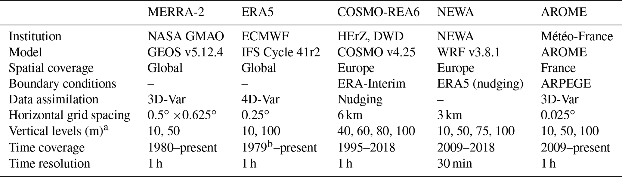
^a Vertical levels refer to the available wind outputs used in the study, not the model levels. ^b ERA5 is to be extended back to 1950.

The two global reanalyses were selected because they are reference datasets in the wind industry and a new state-of-the-art reanalysis in the case of ERA5.

MERRA-2 reanalysis (Gelaro et al., 2017) from NASA's Global Modeling and Assimilation Office and its predecessor MERRA have been much used in the wind industry (e.g. Olauson, 2018, and references therein). It was indeed one of the first reanalyses to produce data at an hourly resolution and output winds not only at 10 m above ground but also at 50 m, closer to turbine hub heights.

ERA5 is the new reanalysis produced by the European Centre for Medium-range Weather Forecasts (ECMWF), as part of the Copernicus Climate Change Service (C3S, 2017). It has been released progressively since 2017 and is much more wind-power friendly than its predecessor ERA-Interim: hourly resolution compared to 6-hourly, wind at 100 m, not only at 10 m, as well as a finer horizontal grid spacing of about 30 km compared to about 80 km. ERA5 is already used for energy applications and shows great improvements over previous reanalyses (e.g. Olauson, 2018; Vortex, 2017; Ramon et al., 2019).

The drawback of global models is their rather low spatial resolution, even for state-of-the-art ERA5. A resolution of a few dozens of kilometres is not able to capture small-scale features which may be important for accurately simulating production at the local scale. That is why some higher-resolved limited-area models are also investigated.

Recent years have seen the development of many regional reanalyses covering Europe. Some were developed within the UERRA (Uncertainties in Ensembles of Regional ReAnalysis) project (UERRA, 2020). In addition, C3S is currently developping the Copernicus regional reanalysis for Europe (CERRA), which will be forced by ERA5 and will cover Europe at a 5.5 km resolution. Alongside the UERRA project, COSMO-REA6 was generated in the framework of the Hans-Ertel-Centre for Weather Research – Climate Monitoring and Diagnostics at the Universities of Bonn and Cologne, and is operated by the German Meteorological Service (DWD). This european reanalysis uses DWD's operational NWP model COSMO with initial and boundary conditions from ERA-Interim reanalysis. It assimilates mostly the same observations as the operational NWP model, using a nudging scheme (Bollmeyer et al., 2015). It was chosen to be evaluated here for its high resolution (6 km), its large spatial coverage over Europe and because it has previously showed good results for surface winds (Kaiser-Weiss et al., 2015).

This study also investigates a completely different type of high-resolution dataset that was specifically designed for wind energy applications: the mesoscale data from the New European Wind Atlas (NEWA consortium, 2020), which is a downscaling of ERA5 at 3 km and 30 min resolution using the Weather Research and Forecasting (WRF) model. A major difference from the previous datasets is that WRF does not assimilate observations. It is driven by ERA5 with a spectral nudging over the domain. WRF was run separatly over 10 domains to cover most of Europe. Another kind of simulations, 50 m microscale simulations were also conducted but are not available for download and thus not investigated.

Finally, the study also investigates the AROME-France NWP model (Seity et al., 2011) for its high resolution over France. AROME is not a reanalysis but an operational model issuing a new forecast every 6 h. Therefore the forecast runs were stitched together to create continuous hourly series. This is done by taking 6 steps in each forecast, see Fig. 1 for a visual explanation. Here the steps +6 to +11 h of each forecast were concatened. It is important to choose carefully the steps. Using the steps +4 to +9 h led to similar conclusions than the steps +6 to +11 h. But steps closer to the analysis should not be used: the analysis and first forecast steps of each run in AROME exhibit large negative biases for wind speeds. This is caused by imbalances in the 3D-Var analysis (for more information on this spin-up issue, see Brousseau et al., 2016). Whatever the choice in steps, the method is not seamless, so jumps are observed every 6 h, at the hours when changing from one run to the other.

Figure 1 Schematic of the reconstruction of a continuous hourly signal by selecting 6 steps (+6 to +11 h here) in each forecast run from an operational NWP model issuing a new forecast every 6 h.

The AROME database used by the author had missing runs, especially in the years 2018 and 2017, which reduced the overall availability of datasets used in the study.

2.2 Wind-speed observations

Wind-speed measurements at levels close to turbine hub heights are difficult to get access to for confidentiality reasons. In this study, measurements were gathered at eight sites:

• Seven from meteorological masts installed for wind farm projects in various locations over France. Top anemometers are ranging from 55 to 90 m above ground. There are also measurements from lower anemometers, useful for filtering the data.

• One from a LIDAR at the SIRTA observatory (Haeffelin et al., 2005) near Paris. The vertical resolution is 20 m and the 100 m level was mostly used.

Information on the measurements (locations, heights, periods and availabilities) are given in Table 2.

Table 2 Information on the wind-speed measurements used in the study: location (approximate for confidential data) and surrounding environment; LIDAR/anemometers heights; measurement time period (1 to 3 years) and availabilities over this period: availability of the observations alone and availability of combined observed and modelled datasets.

The 10 min wind-speed series were manually filtered to remove erroneous measurements such as long periods of zeros or abnormal behaviour of one anemometer compared to the others. Not many anomalies were detected, the measurements were of good quality. The series were then averaged to 30 min. One to three years of measurements are available for each location, with an availability of at least 94 %. The availability declines when considering not only the observation but also the datasets availabilities (because there were missing data in the AROME database used for this study), especially for the masts having data only in 2018 (year having the lowest availability for AROME). Still the overall availability is always above 85 %.

2.3 Wind-power production observations

The lack of wind-speed measurements led to the use of wind-power observations to indirectly evaluate the modelled wind speeds. Two public datasets were used:

• 30 min time series of wind-power production at the regional scale (productions aggregated over the twelve French administrative regions). This dataset is published by RTE, the French Transmission System Operator (TSO). It covers the period from 2013 to 2017.

• Annual energy at the local scale (production from one or a few farms in the same city, summed by year). This dataset is published by Enedis, the main Distribution System Operator (DSO). The dataset contains the years 2011 to 2017.

The contours of the twelve administrative regions can be seen in Fig. 2. They are named by the following acronyms: HDF (Hauts-de-France), NOR (Normandy), BRI (Brittany), IDF (Ile-de-France), GE (Grand Est), PL (Pays de la Loire), CEN (Centre-Val de Loire), BFC (Bourgogne-France-Comté), NAQ (Nouvelle Aquitaine), ARA (Auvergne-Rhône-Alpes), OCC (Occitanie), PACA (Provence-Alpes-Côte d'Azur). IDF and PACA have almost no wind farms (less than 70 MW installed by the end of 2017). Therefore they are aggregated with a neighbouring region (CEN for IDF, OCC for PACA), which leads to studying only 10 regions.

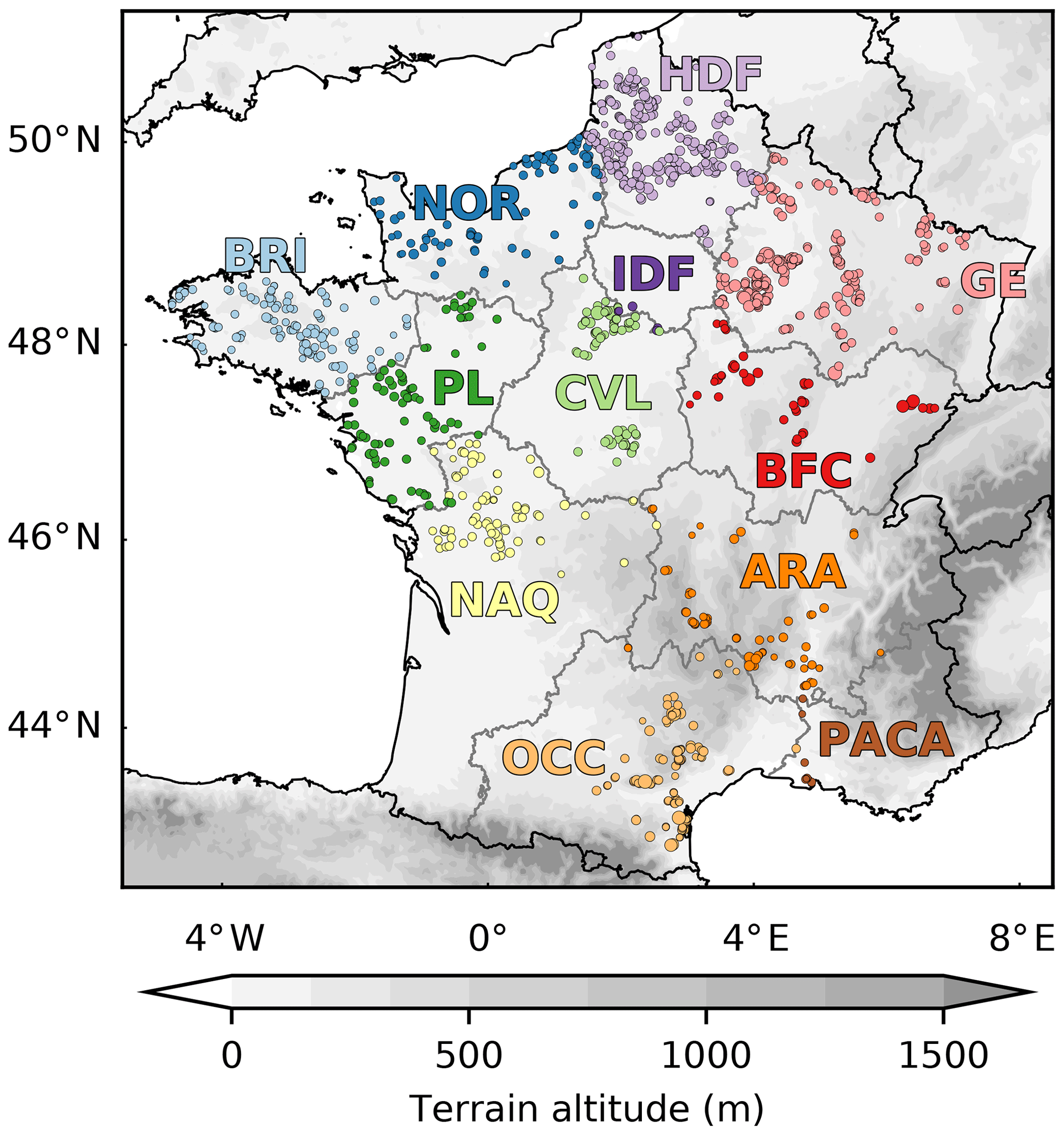
Figure 2 Map of continental France: wind farms installed by the end of 2017 (dots) with colours depending on the administrative region (annotated acronyms, see full names in Sect. 2.3) and orography (grey shades).

Formatted CSV files for these two datasets are available in the Supplement.

2.4 Wind farms information

To be able to simulate wind-power outputs using a physical method (described in Sect. 3.3), the following information was gathered for every wind farm in France:

• geographic coordinates, and corresponding city in the Enedis database (Sect. 2.3),

• commissioning date (and decommissioning date if the farm was dismantled),

• capacity,

• turbine model and associated power curve,

• hub height.

The main source of information was The Wind Power database (TWP, 2020), checked and completed with information coming mainly from Google Maps (satellite views), Open Street Map, French Ministry for ecology and regional authorities (DREAL). The resulting list of all the farms installed before the end of 2017 is available as a CSV file in the Suppplement.

There are 1217 wind farms, whose locations are shown in Fig. 2. The hub height was missing at 199 locations. For these farms, the median height of all farms with the same turbine model was used. The turbines power curves were also obtained from The Wind Power database. Turbines whose power curve was missing in the database (it was the case for 64 farms) were replaced by a turbine with similar characteristics (diameter, rated power, rated speed, cut-in speed, cut-out speed).

3 Methods

This section presents the methods used to extract 30 min wind-speed series from the five studied datasets (Sect. 3.1); to compare observed and modelled wind speeds (Sect. 3.2); to convert wind speeds into wind-power series (Sect. 3.3) and finally to compare observed and simulated power outputs (Sect. 3.4).

3.1 Extracting modelled wind speeds

Wind-speed fields are extracted from the numerical datasets at two or more heights (see Table 1), either directly if the wind speed is an available variable, or computed from meridional and zonal wind components.

At each selected location, wind speeds are interpolated:

1. Spatially to the geographic coordinates using bilinear interpolation, except for the highest resolution datasets NEWA and AROME where the nearest land point was used.

2. In time to a 30 min step (linear interpolation for each available level).

3. Vertically to the anemometer height or turbine hub height using a power law fit on the 2 closest levels. The wind speed w_h at height h is computed from wind speeds w₁ and w₂ at heights h₁ and h₂ using Eqs. (1) and (2):

   $$\begin{array}{}\text{(1)}& {\displaystyle }& {\displaystyle }{w}_{\mathrm{h}}=w_{\mathrm{1}}{\left({\displaystyle \frac{h}{h_{\mathrm{1}}}}\right)}^{\mathit{\alpha }}\text{(2)}& {\displaystyle }& {\displaystyle }\mathit{\alpha }={\displaystyle \frac{\ln \left(w_{\mathrm{2}}\right)-\ln \left(w_{\mathrm{1}}\right)}{\ln \left(h_{\mathrm{2}}\right)-\ln \left(h_{\mathrm{1}}\right)}}.\end{array}$$

   The power law (Eq. 1, e.g. Bailey et al., 1997; Brower, 2012) is often used for extrapolating wind speeds from a single height (typically 10 m) using a fixed value of the wind shear exponent α (typically 0.143, e.g. Troccoli et al., 2018; Lledó et al., 2019). In reality, the shear varies with atmospheric stability, so using an average α introduces errors (Brower, 2012). Here, α is computed at each time step using Eq. (2), which comes from solving the power law for heights h₁ and h₂.

3.2 Comparing modelled and observed wind speeds

At each mast/LIDAR location, the observed 30 min wind-speed series is joined with the wind-speed series extracted from the five numerical datasets. A time step is removed from all time series if any dataset or observation is missing. These time series are used to compute several metrics. The results in Sect. 4.2 show those that were found as the most interesting ones: correlation coefficients, bias and the average diurnal cycles.

3.3 Converting wind speed to power output

Modelled wind speeds are extracted as described in Sect. 3.1 at the coordinates and hub height of every wind farm in France, and then transformed to production using the turbine’s power curve. The theoretical power curve is smoothed with a Gaussian filter in a similar way as Staffell and Pfenninger (2016). The purpose of this filter is to better represent the hourly average output of a whole farm, instead of the instantaneous output of a single turbine. Here the width of the Gaussian filter, which is a function of wind speed w, is $\mathit{\sigma }=\mathrm{0.2}+\mathrm{0.1}\times w$ m s⁻¹. It is smaller than in Staffell and Pfenninger (2016) because the productions are averaged over 30 min instead of an hour. This filter changes the power curve mainly at high wind speeds in order to smooth the sharp decrease of theoretical power curves at the cut-out wind speed.

The resulting 30 min wind-power time series are too optimistic because they do not take into account any loss. Removing losses from gross production to get “real-life” net production is a very important part of the wind resource assessment methodology and under-estimating the losses have led to over-estimating the resource in many past projects (Brower, 2012, see Sect. 16.6). In simulations however they are not always considered. It is not a problem with statistical methods that train on observed production but it is with purely physical methods. Note that methods combining physical modelling and bias corrections may take into account losses in a hidden way. For example in Staffell and Pfenninger (2016), the wind speed bias correction fit using observed national capacity factors corrects not only the bias of the underlying MERRA data but probably also the losses that are not accounted for in their virtual wind farm model.

Losses come from:

1. non-optimal conditions that make the turbines produce less than theoretically: lower air density than reference, turbulences, misalignment to the wind flow, etc. (according to Brower (2012), typical values range from 2 % to 5 %), and also dirty blades and other environment impacts [1 % to 6 %],

2. electrical losses of all components of the wind farm [2 % to 3 %],

3. stops due to failures or to maintenance operations [2 % to 10 %],

4. wake effects inside the wind farm or caused by a very close farm [3 % to 15 %],

5. curtailments, i.e. voluntary reduction of power output because of grid congestion or to reduce environmental impacts such as noise or bat fatalities [0 % to 5 %].

The overall loss factor has a typical value of 18.5 % within a wide range from 7.8 % to 37 % (Brower, 2012). It is site-dependent but also varies in time as external factors change and turbine performance tends to decrease with age (Staffell and Green, 2013).

In this study the loss factor λ is taken as 15 % as a most probable value (the simulated wind-power series are multiplied by 0.85). This choice was confirmed by local energy outputs of wind farms in the vicinity of the measurement masts: at places with no wind-speed bias, using λ=15 % enabled to remove the wind-power bias. However this value is surely not exact for all wind farms. For further discussion, the results were also computed for several λ ranging from 10 % to 30 %.

3.4 Comparing simulated and observed wind-power outputs

The power-output time series are aggregated in two different ways:

1. Spatial aggregation over regions. These regional times series are compared to the RTE database. As for the wind-speed time series, correlation coefficients, bias and diurnal cycles are investigated.

2. Spatial aggregation over cities and time aggregation over the years. These annual sums of energy are compared to the Enedis database, in terms of bias only since they are not time series.

The spatial aggregation at the local scale takes into account that a city may correspond to several wind farms but also that a wind farm may be scattered over several cities (having to sum a small number of cities from the Enedis database). A year is discarded if the installed capacity of the city changed during the year (if a farm was installed or dismantled). The number of local aggregates varies from 386 in 2011 to 651 in 2017.

The results of these comparisons are presented in Sect. 4.3.

4 Results

After highlighting an issue discovered in ERA5 wind speeds, this Section presents the results from the direct validation using wind-speed observations (Sect. 4.2) and from the indirect validation using power and energy observations (Sect. 4.3).

4.1 Issue in ERA5 diurnal cycles

The author discovered an issue with the diurnal cycles of wind speeds in ERA5. The wind speeds at 10 m, 100 m and also on lower model levels, exhibit gaps at 10:00 UTC and following hours and similarly but in a lesser extent at 22:00 UTC. The wind deficit at 10:00 UTC may be larger than 0.5 m s⁻¹ on average. Examples are given below, in Sect. 4.2 with average diurnal cycles drawn in Fig. 3b–h.

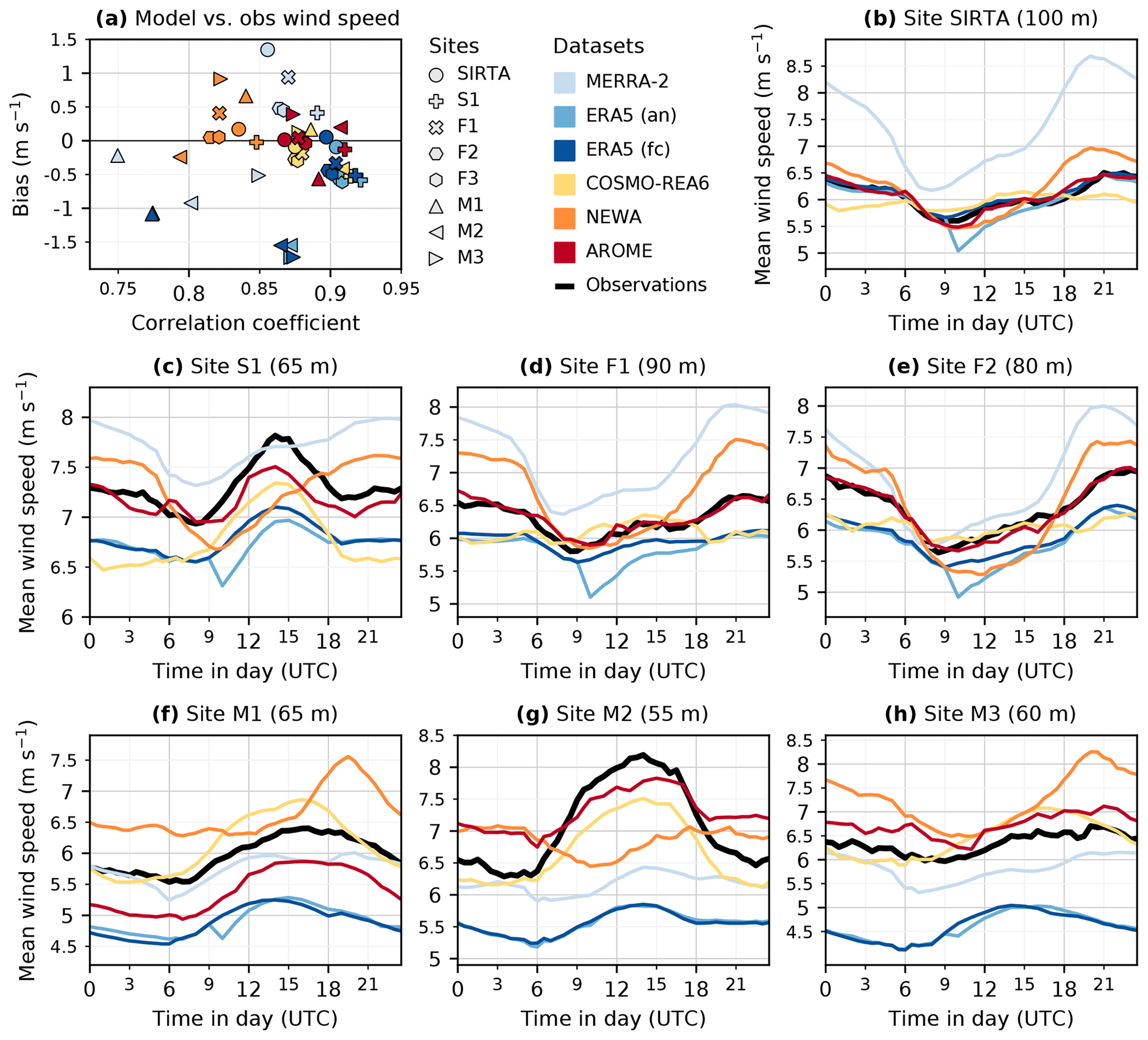
Figure 3 Comparison of modelled and measured wind speeds at 8 locations. (a) For each location (identified by marker style) and each model (identified by marker colour): bias (model – observation, on the y-axis) versus correlation coefficient (on the x-axis) of the 30 min time series. The time period depends on the location: see Table 2. (b–h) Average diurnal cycles of the observed (in black) and modelled (in colours) wind speeds at all locations except F3 which is extremely similar to F2 (same time period and very close locations). See location characteristics in Table 2.

The issue was reported to ECMWF which acknowledged the problem, which is linked to the assimilation process, affects mostly low latitude oceanic regions but also Europe and North America, and is not possible to correct (ERA5 data documentation, 2020). The issue appears at both 10:00 and 22:00 UTC but is more visible in convective atmospheric conditions thus appearing mostly at 10:00 UTC, during the day, over continental France.

To address this issue, ERA5 forecasts (denoted “fc” hereafter) were downloaded and studied in addition to the usual analysis data (denoted “an”). The forecasts do not exhibit the issue at 10:00 and 22:00 UTC but there may be jumps at 07:00 and 19:00 UTC when moving from one forecast stream onto the next. These jumps are small or not visible over continental France.

4.2 Wind-speed validation

The wind-speed inter-comparison at the eight measurement locations are shown in Fig. 3: Fig. 3a summarizes the bias and correlation at all locations; Fig. 3b–h show the average diurnal cycles at all locations except F3, which is very similar to F2.

Figure 3a shows that AROME (in red) and COSMO-REA6 (in yellow) are the only two datasets that have small biases (absolute value below 0.6 m s⁻¹) and high correlation coefficients (above 0.86) at all locations. AROME represents quite well the shape of the observed diurnal cycle in simple terrains (sites SIRTA, F1–F3) and shows only small departures in more complex environments: either a general bias (sites M1 and M3) or a too small amplitude (sites S1 and M2). COSMO-REA6 has often slightly better correlations than AROME (above 0.87) and small but rather negative biases. But it is struggling with diurnal cycles: at the three locations in flat environments, the cycles are flatter than the observed ones, with a negative bias at night. This can be linked to the issue detailed by Heppelmann et al. (2017): difficulties with stable conditions, with nocturnal low-level jets and with vertical mixing after sunrise, originating from the boundary layer turbulence scheme in the COSMO model. In the more complex environments (sites S1 and M1–M3), diurnal cycles have a form closer to the observed ones, but it could be because the measurements in these locations happen to be at lower levels (below or close to 60 m), which are less affected by the issue.

ERA5 (in dark blues) shows the highest correlations (mostly above 0.9) except in mountainous areas (sites Ms depicted with triangles in Fig. 3a), with a minimum of 0.77 at site M1. ERA5 exhibits negative biases around −0.5 m s⁻¹ in flat areas and larger in mountainous regions (down to −1.7 m s⁻¹ at site M3). Using the forecasts instead of the analysis has little impact on the correlations and biases. The main difference between the two is seen in the diurnal cycles: while the analyses exhibit a sharp decrease between 09:00 and 10:00 UTC, the forecasts do not. The wind deficit lasts several hours, up to 19:00 UTC. The deficit is larger in northern regions and does not appear at one site, M2, which is in a valley surrounded by high mountains in Southern France, close to the Mediterranean Sea. Apart from this issue, ERA5 shows very good skills with the diurnal cycle, even in complex environments: there is a bias but the form is good.

MERRA-2 (in light blue) has good correlations at sites with simple terrain (above 0.85) but over-estimates the wind speed, especially at night. The bias reaches 1.35 m s⁻¹ at SIRTA and 0.94 m s⁻¹ at site F1. At the mountainous sites, MERRA-2 has negative biases (minimum of −0.93 m s⁻¹ at site M2) and the correlations drop (down to 0.75 at site M1). The diurnal cycles are not well depicted, especially at the sites with complex terrain.

NEWA (in orange) has biases ranging from −0.24 to 0.91 m s⁻¹, with a rather positive tendency. Biases are smaller than those of the large-scale reanalyses in most cases and comparable to the high-resolution datasets. The correlations however are much worse. With a median of 0.82, NEWA has the lowest correlation at all sites except M1 where ERA5 and MERRA-2 are worse. The fact that NEWA has 30 min outputs while the other datasets are linearly interpolated from hourly outputs may be a disadvantage for this metric: the higher 30 min variability being not in phase with the observations, degrades the correlation coefficient. The low correlations are also explained by the diurnal cycles, which show that physical processes in the boundary layer are not well reflected by NEWA. The diurnal cycles are far from the observed ones with sometimes inversed variations (M2). All sites exhibit a positive bias at night and a seasonal analysis finds larger biases in winter (not shown). An interesting example is site S1, where NEWA has a bias close to zero: the diurnal cycle shows that there is in fact a positive bias at night, offset by a negative bias during the day. The modelled diurnal variations are not in phase with the observed ones.

This wind-speed analysis is limited by the small number of sites, which impedes general conclusions. A wider analysis is conducted using wind-power data.

4.3 Wind-power validation

The first approach using RTE 30 min time series informs about the dynamics of the simulations. Figure 4 shows the comparison between observed and simulated productions aggregated at the regional scale: Fig. 4a summarizes biases and correlations for France and all regions; Fig. 4b–e shows the average diurnal cycles for France and three example regions. Wind farms are mostly located in HDF and GE. Each of these two regions has almost a quarter of the national installed capacity. Their diurnal cycles are very similar to the country's cycle, drawn in Fig. 4b, and therefore are not shown here. The third, fourth and fifth regions (between 10 % and 7 % of the national capacity) are OCC, CEN and BRI. They show rather different cycles, which are shown in Fig. 4e, d and c.

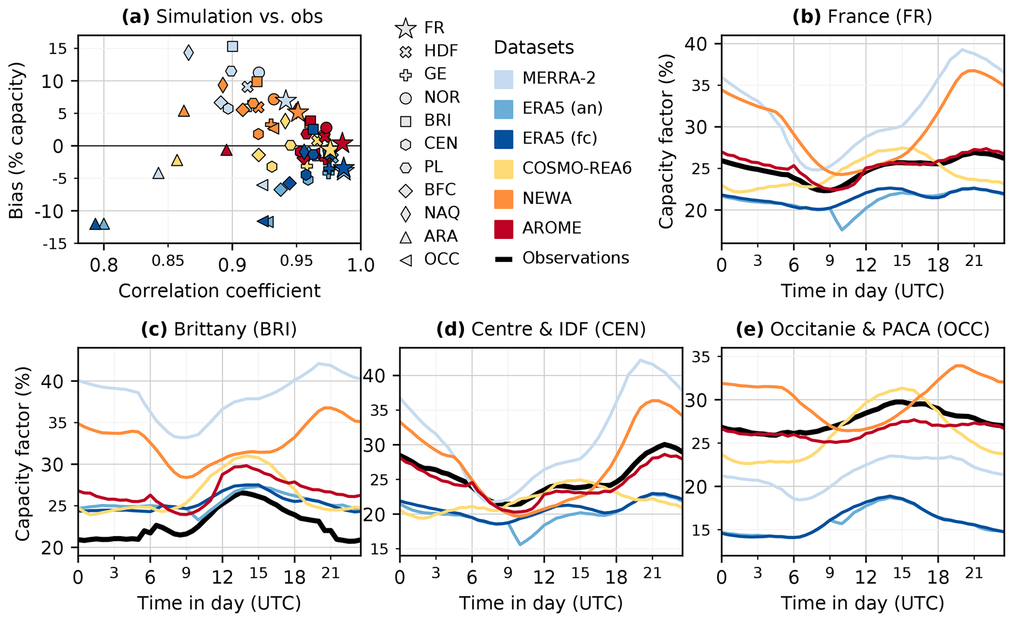
Figure 4 Comparison of modelled and measured wind-power production for France in 2015. (a) For each region (identified by marker style) and each model (identified by marker colour): bias in percent of the installed capacity (model – observation, on the y-axis) versus correlation coefficient (on the x-axis) of the 30 min wind-power time series. See region map in Fig. 2. (b–e) Average diurnal cycles of the observed (in black) and modelled (in colours) wind-power capacity factors for the whole France (b), Brittany (c), Centre summed with Ile-de-France (d) and Occitanie summed with PACA (e).

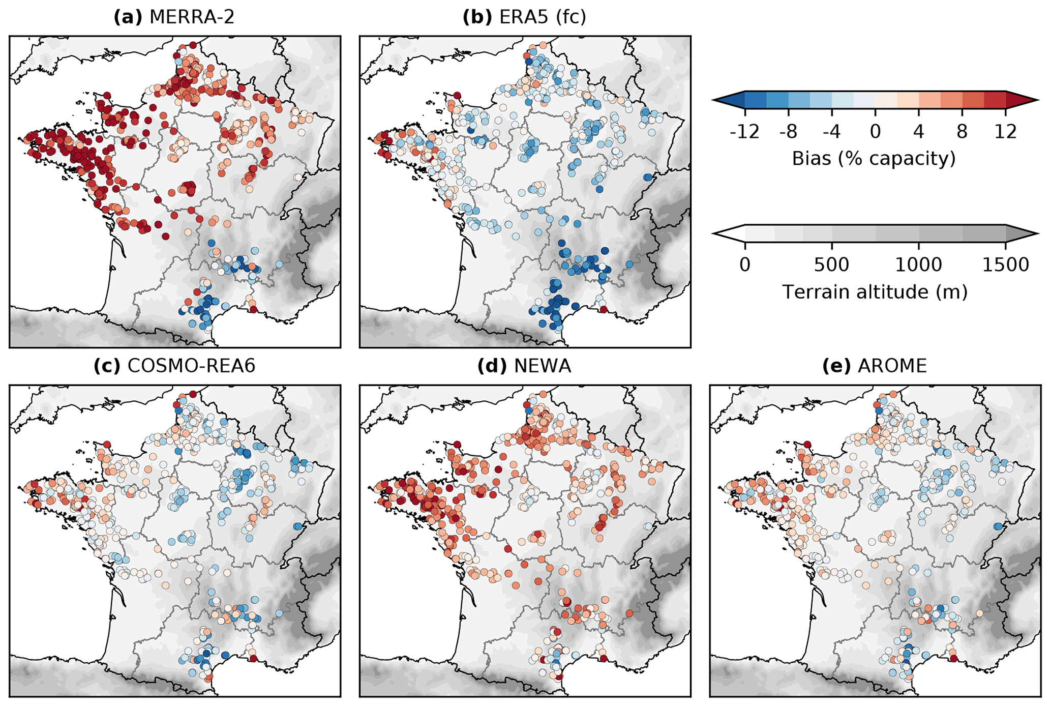
Figure 5 Local biases of wind-power production simulations based on MERRA-2 (a), ERA5 (forecasts) (b), COSMO-REA6 (c), NEWA (d) and AROME (e), compared to Enedis database at city scale. Bias (model – observation) in average power expressed in percent of the city installed capacity. Year 2015, loss factor of 15 %.

This regional approach is complemented by local (but annual) information using the Enedis database. Figure 5 shows the local biases. A positive (resp. negative) bias in red (resp. blue) means that the model-based simulation overestimates (resp. underestimates) the observed production. Some large local errors in Fig. 5 may originate from errors either in the Enedis database or when linking the Enedis database to the list of wind farms, or from an anomalous observed production of an under-performing wind farm. The interest is not about those isolated singular points but about the general pattern over France and in particular inside each administrative region.

The following scores and figures are given:

• For a loss factor of 15 %. This assumption is discussed in Sect. 5.1.

• For year 2015 as an example; they are similar for all available years, see discussion in Sect. 5.2.

MERRA-2 has the largest biases (6.9 % for France) and the lowest correlations (0.94 for France) (Fig. 4a). The diurnal cycles show that the overestimation comes mostly from the night time (Fig. 4b). At the local scale (Fig. 5) the production is largely overestimated in the northern part of France: the median bias at the local scale is 9.2 % of the installed capacity, whereas the average production of a wind farm is around 25 % of the installed capacity. Therefore, if computed in terms of the local observed production, the median bias in northern regions is 39 %. In the southern mountainous regions on the contrary, MERRA-2 largely underestimates the production: the median bias is −5.5 % (−22 % of the observed production). This under-estimation is also seen in the diurnal cycles of the corresponding regions: OCC & PACA in Fig. 4e and ARA (not shown).

ERA5 has the highest correlations for France (0.987) and all regions except in mountainous areas (ARA, OCC, and also BFC) (Fig. 4a). The diurnal variations are well represented (except for the problem at 10:00 UTC and ahead, in the analysis). The biases are mostly negative (−3.4 % for France) and very large in the mountains (Fig. 4). At the local scale, the median bias is −2.0 % in the northern regions and −10.9 % in the southern mountainous regions (resp. −8 % and −48 % of the observed production). Some positive biases appear along the coasts, especially in Brittany (Fig. 5).

For NEWA, the position is slightly different than with the wind-speed validation, where it had the worst correlations but little bias. Here the correlations are a little better than for MERRA-2 but the bias is large (5.1 % for France) (Fig. 4a). The tendency towards positive bias is enhanced when going to production, probably because of the large over-estimations at night. The local biases are positive 90 % of the time; the median is 5.4 % of the installed capacity (23 % of the observed production) (Fig. 5).

AROME and COSMO-REA6 have very high correlations (0.986 and 0.976 for France). They are just behind ERA5 except in mountainous regions where they do better (Fig. 4a). Diurnal cycles are well represented by AROME but not by COSMO-REA6 which tends to overestimate the production during the day and underestimate it at night (Fig. 4b). They both have low biases at the local scale (Fig. 5), with a median bias close to zero and a distribution slightly skewed towards positive (resp. negative) values for AROME (resp. COSMO-REA6). The first and third quartiles of the local biases are −2.1 % and 3.2 % for AROME; −3.5 % and 2.5 % for COSMO-REA6.

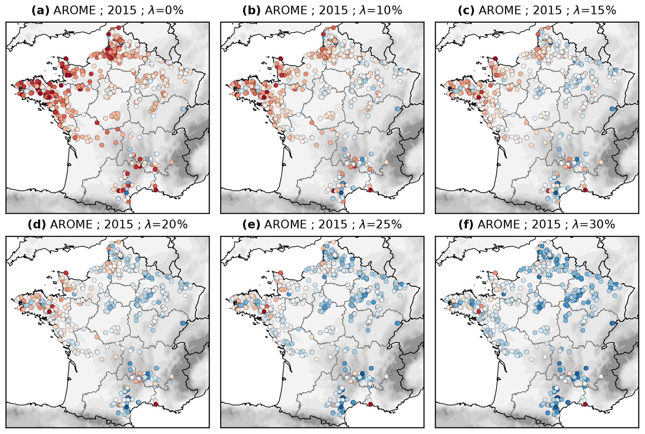
Figure 6 Local biases of wind-power production simulations based on AROME for year 2015 for loss factors varying from 0 % to 30 %. Same scale as Fig. 5.

5 Discussion

This Section discusses the results: the loss factor and its impact on the bias scores in Sect. 5.1, the inter-annual variability in Sect. 5.2 and consistency with previous studies in Sect. 5.3.

5.1 Loss factor

An assumption was made for the loss factor. λ=15 % was chosen as a most probable value but is not the truth. This impacts the bias scores but do not fundamentally change the conclusions. Simulating with a loss factor of 10 % (resp. 20 %) instead of 15 % would add (resp. subtract) about 1.5 % to all biases. This is not such a big change, because biases are expressed in % of the installed capacity while the loss factor is expressed in terms of gross production whose average value is usually below 30 % of the installed capacity. Examples of local biases with AROME for various loss factors are shown in Fig. 6. Therefore in the results, zero, −2 % or +2 % are rather equivalent bias scores because it is not possible to know the actual amount of loss at each farm. With such small local biases as those found with AROME or COSMO-REA6, the error due to wind-speed biases in the numerical datasets reaches the same order as the uncertainty about the physical modelisation of losses. It is impossible to say that one dataset is better than the other. They both create realistic simulations. But the other datasets have much larger biases, in particular MERRA-2, which has still mostly positive biases in northern France even with a loss factor of 30 %.

When comparing all datasets, similar behaviours appear in some areas. For example in the northern part of CEN and the western part of GE, all datasets have lower biases (smaller positive biases or larger negative biases) than in other northern areas. It could be that these field areas are flatter than the numerical models expect. If the surface roughness is overestimated, the wind speed would be underestimated.

Another region of interest is Brittany (BRI) where there are many positive biases at the local scale. It is the only region for which all datasets, even ERA5, overestimate the aggregated production. Part of the explanation may be that wind farms in this region experience much larger losses. In Brittany, we need λ=25 % or 30 % to set most AROME local biases to zero for example (Fig. 6). The regional diurnal cycles in Fig. 4c show an interesting phenomenon at night. You can see steps in the observed production (black line) in the morning and in the evening. They correspond to ending and starting hours of night-time curtailment: the turbines are slowed down between 22:00 and 07:00 LT (local time) (i.e. between 20:00 and 05:00 UTC in summer and between 21:00 and 06:00 UTC in winter) to reduce noise impacts on neighbour inhabitants. A seasonal annalysis (not shown) indicates that the curtailment is particularly important in the winter. These curtailments contribute to the overestimations at night but do not explain everything. There could be other losses, for example due to the rather old age of the farms in this region. Part of the overestimation may also come from numerical models underestimating wind speeds in this hilly region encircled by the sea. In this study however, there was unfortunately no available wind-speed observation in Brittany to evaluate the relative contributions of losses and wind biases.

5.2 Inter-annual variability

The results were presented for year 2015 but were conducted for all available years. They all look the same (example with ERA5 in Fig. 7), except that the number of local aggregates increases.

Figure 7 Local biases of wind-power production simulations based on ERA5 (forecasts) for years 2011 to 2017, except 2015 shown in Fig. 5b. Same scale as Fig. 5.

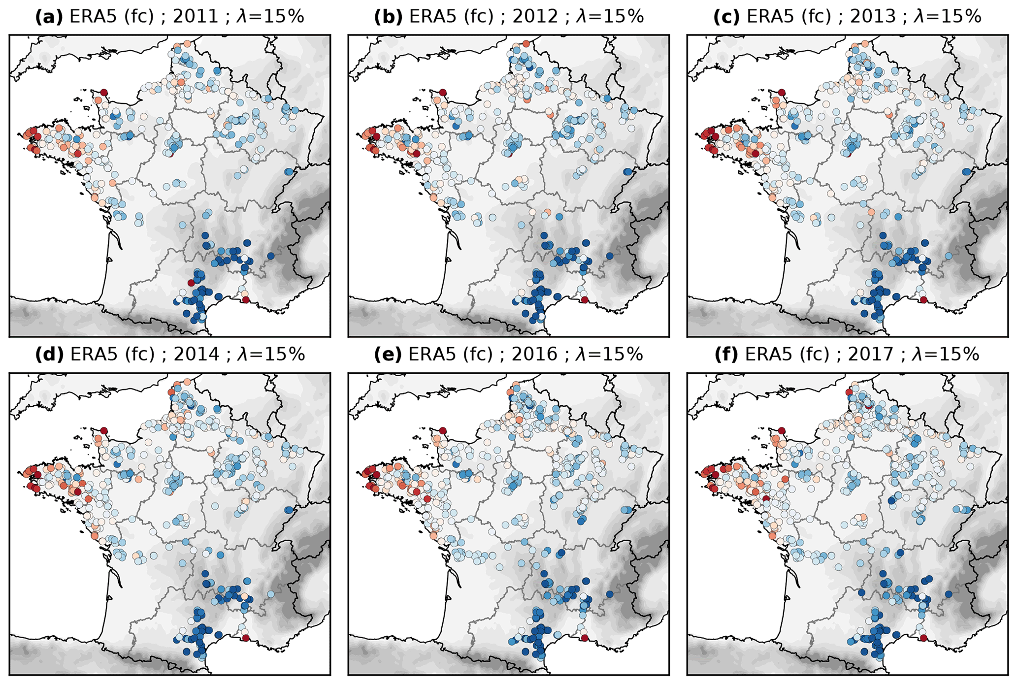
The period of the study is very short considering the large variability of wind speed on inter-annual to decadal time scales. In fact this period is biased low when compared with past decades (and especially the period around 2000, which saw much higher wind speeds in northern France, related to a very positive phase of the North Atlantic Oscillation). 2015 is the only year above the long-term average and 2016–2017 are very low years. To be thourough one would have liked to see also a very high year in this period. But the fact that the results are the same for all years, especially 2015 and 2017, is reassuring about the robustness of the conclusions in the long-term.

5.3 Consistency with previous studies

For MERRA or MERRA-2 simulations aggregated at the national levels in Ninja, Staffell and Pfenninger (2016) found correction factors indicating negative wind-speed biases in southern Europe and positive biases in countries bordering the North, Baltic and Celtic seas. Monforti and Gonzalez-Aparicio (2017) found concordant results for MERRA-based simulations with their analysis on sensitivity to wind speed. The present study at the local scale with MERRA-2 (Fig. 5a) shows how this line dividing Europe is crossing France, separating the Mediterranean region from the western-northern regions. For France, a unique bias correction fit at the national level is therefore not adapted.

Olsen et al. (2019) presented a validation of NEWA, and the underlying ERA5 data, using wind-speed measurements from Vestas, which is part of the NEWA consortium. There were almost 300 masts over Europe (including 30 in France but the results are only shown on the whole set). Their results are that ERA5 under-estimates the wind speed: average bias of −1.5 m s⁻¹, the bias increasing with the ruggedness index (RIX). It is in agreement with what is observed in this study. For NEWA, Olsen et al. (2019) finds no bias on average (bias of 0.02 m s⁻¹), but there is a rather positive bias in flat terrains (0.21 m s⁻¹, on average for masts with RIX = 0 %) and a negative one for complex terrains (−0.25 m s⁻¹, on average for masts with RIX > 2 %). Moreover simulations using a generic turbine power curve show that, even though there is no wind-speed bias on average, the power generation is overestimated by 6 % on average (11 % in flat terrains). This study shows very compatible results. One difference is that two of the mountainous sites have large positive biases, not negative, but they still have absolute biases lower than ERA5. The bias was also seen enhanced when going to production. The median local bias of 5.4 %, lower in mountainous areas, is in line with Olsen et al. (2019) findings.

This evaluation tends to advocate towards NWP model with their own assimilation system, such as COSMO and AROME, rather than dynamical downscaling. Their is also a question about the WRF parameterizations chosen for NEWA. The main sensitivity experiment that was conducted to choose the parameterizations was using masts measurements located only in Northern Europe and at locations either offshore or close to the sea (Witha et al., 2019). Maybe this choice was not very appropriate for France.

Evaluating model skills is not an easy task, even when proper observations are available, because many metrics are possible and skills depend on the application. The study shows that considering only averaged metrics, such as bias, is not sufficient. It could not have detected the assimilation problem in ERA5 nor the turbulence problem in COSMO-REA6. The NEWA validation using average wind-speed bias did not detect the offset between night-time overestimation and day-time underestimation of wind speeds. Looking at diurnal cycles is really interesting, not only because they reveal hidden intra-day biases, but also because they are a good measure of how well the boundary layer physical processes are parameterized in the models. Drawing separate diurnal cycles per seasons (not shown here) may be even more revealing because many issues, especially those linked to convection, impact differently winter and summer times.

6 Conclusions

When it comes to simulating wind-power production, no numerical weather model is perfect but much progress has been made over the last years. Considering large-scale global models, the new reanalysis ERA5 shows very good skills. This study over France shows that it outperforms MERRA-2, which was largely used in the wind industry so far, with lower bias, higher correlation, and better diurnal variability. Yet, some problems appear. Firstly an assimilation problem that creates a negative bias in wind speed at 10:00 UTC, takes hours to recover and therefore impacts the diurnal cycle. Correcting this problem (for example by using the forecast instead of the analysis) may be very important, depending on the application. Secondly ERA5 underestimates the wind speeds and this may lead to some major underestimation of the wind energy production, especially in areas with complex topography, if not corrected. Some higher resolution models, such as AROME or COSMO-REA6 show very good skills too, reducing the bias and increasing the correlation in complex topography. Yet, COSMO-REA6 has wrong diurnal variations probably due to its turbulence scheme and AROME is not very homogeneous because it is not a reanalysis. High-resolution models are not all equally skilled: the mesoscale data from NEWA have disappointing results compared to the other two models and even compared to ERA5 on which it is based.

For various applications at EDF, the present study led to implementing a method using ERA5 reanalysis (fc) with a local wind-speed correction trained with either AROME or COSMO-REA6. The simple physical method makes it possible to simulate any future farm when no observation (neither wind speed nor production) is available, given only the following information: geographical coordinates, hub height, theoretical power curve and loss assumptions (the losses are implemented in a different way than in this study in order keep capacity factors ranging from 0 to 1). The use of ERA5 as the main data source enables to simulate over several decades (starting from 1950 when ERA5 extension will be available), which is necessary for some applications. For prospective studies on a larger scale, it is also possible to use this method using a bottom-up approach, i.e. aggregating at the regional or national scale the local simulations made for a whole fleet of future wind farms.

New upcoming reanalyses could be evaluated in a similar way in the future, for example the Copernicus regional reanalysis for Europe (based on ERA5), and a new version of COSMO-REA6 using ERA5 instead of ERA-Interim as boundary conditions and a more recent version of the COSMO model, which could have an improved turbulence scheme.