 | 05 Aug 2021
Towards a reproducible snow load map – an example for Austria
Harald Schellander
Michael Winkler
Tobias Hell
The European Committee for Standardization defines zonings and calculation criteria for different European regions to assign snow loads for structural design. In the Alpine region these defaults are quite coarse; countries therefore use their own products, and inconsistencies at national borders are a common problem.
A new methodology to derive a snow load map for Austria is presented, which is reproducible and could be used across borders. It is based on (i) modeling snow loads with the specially developed Δsnow model at 897 sophistically quality controlled snow depth series in Austria and neighboring countries and (ii) a generalized additive model where covariates and their combinations are represented by penalized regression splines, fitted to series of yearly snow load maxima derived in the first step. This results in spatially modeled snow load extremes.
The new approach outperforms a standard smooth model and is much more accurate than the currently used Austrian snow load map when compared to the RMSE of the 50-year snow load return values through a cross-validation procedure. No zoning is necessary, and the new map's RMSE of station-wise estimated 50-year generalized extreme value (GEV) return levels gradually rises to 2.2 kN m−2 at an elevation of 2000 m. The bias is 0.18 kN m−2 and positive across all elevations. When restricting the range of validity of the new map to 2000 m elevation, negative bias values that significantly underestimate 50-year snow loads at a very small number of stations are the only objective problem that has to be solved before the new map can be proposed as a successor of the current Austrian snow load map.
- Article
(2607 KB) - Full-text XML
- BibTeX
- EndNote


The current European standard for structural design – Eurocode EN 1991-1-3 (CEN, 2015) – defines rules to calculate acceptable snow loads on constructions and buildings. It is based on snow load maps for different climate regions, defining snow load zones. Within these zones a linear or quadratic “elevation–snow load relationship” is used to calculate sk, the so-called characteristic snow load on the ground, which in turn is based on an annual probability of exceedance of 0.02 and referred to as the return level of snow load (in kN m−2) of a 50-year return period. EN 1991-1-3 defines, for example, an “Alpine region” reproduced in Fig. 1, where , with Z being the zone number as defined in the legend of Fig. 1 and A being elevation of the location for which sk should be calculated (A≤1500 m a.s.l.). All strategies outlined in EN 1991-1-3 for how to consider the various influences of roof shapes, thermal properties, wind drift, etc. are ultimately connected to sk, making it the most crucial snow-load-related quantity for structural design.
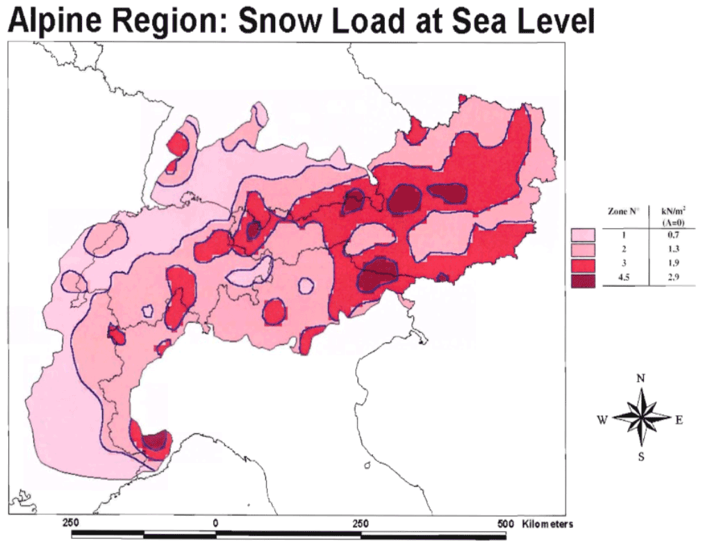
The aim of this default snow load definition by the European Committee for Standardization (CEN) is “to eliminate or reduce the inconsistencies of snow load values in CEN member states and at borderlines between countries” (CEN, 2015). It results from comprehensive research work of the late 1990s under contracts of the European Commission (Sanpaolesi et al., 1998, 1999). However, Annex C of EN 1991-1-3, where maps and sk relations are defined, has an informative character, not a normative. Member states can define their own maps, as has already been done before the Eurocode suggestions were developed. In Austria, ÖNORM B 4013, (ON, 1983), for example, already provides a map with much more attention to detail than the Eurocode map. Snowfall in Austria is characterized by a complex climatic setting (Auer et al., 2006) as well as the country's structured topography, leading to small-scale shading and enhancement effects for precipitation (e.g., Wastl and Zängl, 2010), frequent valley inversions, and spatially and temporally highly diverse snow lines (e.g., Unterstrasser and Zängl, 2006). In 2006, when the Austrian standard was based on Eurocode for the first time (ON, 2006), the zoning was adopted to make use of the abovementioned relation. Still, the richness of detail of the map was kept rather than using the coarse Eurocode suggestion (reprinted in Fig. 1; details on the development of the Austrian snow load standard are given in Winkler et al., 2020). Austria's neighbors also use their own snow load maps (e.g., DIN, 2019; SIA, 2020; Autonome Provinz Bozen Südtirol, 2002). Inconsistencies at borderlines between countries are very common. The underlying methods of how snow load maps are developed are roughly comparable: statistical analysis of yearly snow depth maxima using extreme value theory, assigning snow densities, regionalization into climatic snow load regions, etc. (the final draft for the coming Eurocode – CEN, 2020, Annex A.3 – provides guidance), but in the details they are very different. Not least, some of these methods may be subjective and not reproducible (e.g., the drawing of the zones), and others might not be applied in a transparent way (e.g., how and why certain snow density assumptions are made). In this respect CEN's Eurocode EN 1991-1-3 (CEN, 2015) currently misses its target (cf. Croce et al., 2019). Furthermore, the current Austrian standard (ASI, 2018) suffers from an old database that largely ends in the 1980s. Besides the mentioned methodical inadequacies concerning most standards, this particularly offers motivation to update the Austrian snow load map (see also CEN, 2020, Annex A.5).
Here we propose a novel methodology which will lead to an updated snow load map for Austria. It is based on updated snow data and on transparent and reproducible methods described in Sect. 2 that could also be used in other countries. Section 3 provides comparisons to another methodical candidate and the current Austrian snow load standard as well as accuracy measures. Concluding remarks and an outlook on possible future developments are given in Sect. 4.
Long-term snow depth data from 2740 stations in Austria and nearby (ca. 50 km) in Germany, Switzerland, Italy and Slovenia were collected. The data were corrected in many ways. Only a few tasks are shortly outlined here for a more comprehensive illustration the reader is referred to the report on the “Schneelast.Reform” project (Winkler et al., 2021b). A common observational issue is to simply add new snow values over several days and use that as snow depth. Such cases were detected by comparing snow depths with empirical elevation-related thresholds. The wrong values were then corrected by assuming an empirical densification rate with the aid of neighboring stations. One of the essential prerequisites of the Δsnow model is a gapless snow depth record. For Austrian stations gaps up to 31 consecutive days were filled using the dual-layer snow model SNOWGRID (Olefs et al., 2013, 2017). To replace missing observations at a station, the corresponding snow depth time series of the closest SNOWGRID grid point (maximum distance 0.71 km) was linearly interpolated to the observations confining the gap. Years with gaps larger than 31 d were rejected. For non-Austrian stations years with data gaps longer than 6 d were not used, up to 6 d the snow depth records were filled by linear interpolation. About 1.8×10⁷ daily snow depth values were used; 8400 (0.05 %) were filled by the procedure described. At two stations a new snow depth maximum for one season was created; at one station the above-described gap filling led to the second-highest value in one season. Finally, snow depth series from 897 stations fulfilled the following requirements:
-
at least 30 years of regular daily snow depths between 1960 and 2019;
-
latest year with data is 2009 or later;
-
no multiple stations within 0.1∘ latitude or longitude and within 100 m elevation difference.
The stations lie between 118 and 3109 m elevation (median: 655 m; Fig. 2), and the record lengths are between 30 and 59 years, with a median of 49 years. They cover most of the eastern Alps; see Fig. 3.
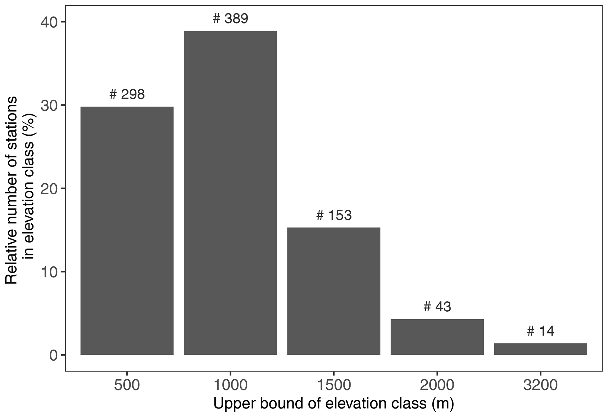
Figure 2Relative number of stations in elevation classes, with the actual number on top of each bar (897 stations).
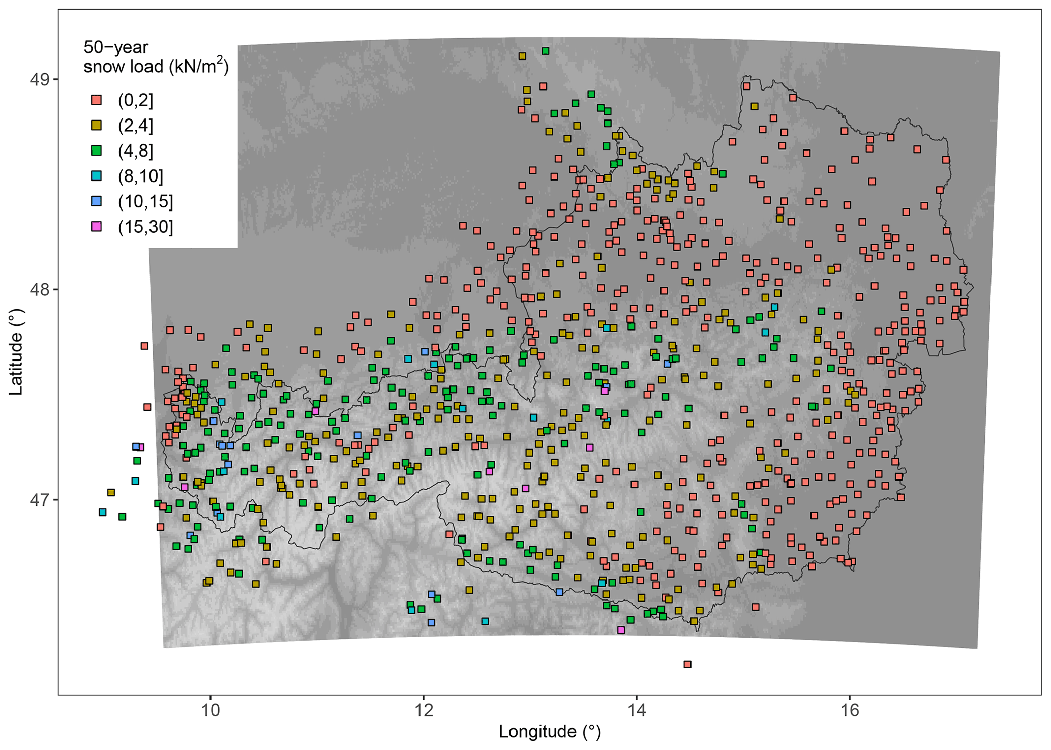
Figure 3Values of 50-year snow load return from Δsnow-modeled yearly maxima locally fitted to a GEV distribution for all 897 stations. Elevation is given in grayscale from 100 m (dark) to 3800 m (light).
The newly derived set of snow depth data series is the most comprehensive of its kind in Austria. No other snow dataset contains so many records with regular data at daily resolution for so many years – the most important prerequisites for deriving return levels of snow load. Individual single-day snow depth values are less important than completeness and capturing the yearly maxima as accurately as possible. Snow depth data still provide the base for snow load modeling rather than snow load or water equivalent observations, for which only too short, too sparse and too irregular series exist (cf. Winkler et al., 2021a). However, using snow depth as a starting point necessitates the simulation of snow mass by applying a snow (density) model.
2.1 Snow model
Former developments of snow load standards used constant snow densities or parameterized elevation, snow type and/or age dependencies. An overview is given in Sanpaolesi et al. (1998). The methods are very heterogeneous. European standards also suggest snow densities (e.g., CEN, 2015; ASI, 2018). Given the complex layered structure and viscoelastic behavior of snow as a porous material very close to its pressure melting point, these simple density assumptions fall short. Also “empirical regression models” (cf. Winkler et al., 2021a) like Jonas et al. (2009), Sturm et al. (2010) and Guyennon et al. (2019) are not applicable since they fail to model yearly maxima sufficiently well (Winkler et al., 2021a). On the other hand, sophisticated “thermodynamic snow models” like SNOWPACK (Lehning et al., 2002) or Crocus (Vionnet et al., 2012) need meteorological forcing that is not available for those long-term snow data.
To simulate proper snow loads for the snow depth records described above, Δsnow was developed (Winkler et al., 2021a; Schellander and Winkler, 2020). It is a semi-empirical layer-resolving snow model which exclusively needs regular snow depth series as input to model respective series of snow loads. Winkler et al. (2021a) show that yearly snow load maxima can be modeled with a very low bias and a root mean square error of 0.36 kN m−2, which is much more accurate than empirical regression models or using categorized or constant snow densities. The Δsnow model was applied to the daily snow depth series described above, leading to 897 snow load series used for spatial interpolation.
2.2 Spatial extreme value statistics
The characteristic snow load on the ground (sk) can be calculated by assuming that yearly sk maxima follow a generalized extreme value (GEV) distribution (Coles, 2001). Among many other environmental parameters, this has been already proven to be reasonable for snow depth (e.g., Marty and Blanchet, 2012; Nicolet et al., 2018). Given the strong correlation between snow depth and snow load, the GEV has also successfully been used for the estimation of extreme snow loads (Le Roux et al., 2020). However, there are also other choices like the lognormal distribution (Mo et al., 2016; DeBock et al., 2017).
Eurocode EN 1991-1-3 (CEN, 2015) demands a spatial representation of sk. Different kriging variants were already used to interpolate snow load extremes for hazard mapping in Canada (Hong and Ye, 2014) and Croatia (Perčec Tadić et al., 2015). There exist, however, more appropriate methods for the spatial modeling of extremes, all trying to model the three parameters location (μ), scale (σ) and shape (ξ) of the GEV with spatially varying covariates. Another typical choice for modeling spatial extremes are max-stable processes (Haan, 1984), which were used by, for example, Schellander and Hell (2018) for snow depth. With max-stable processes also the spatial dependence of extremes has to be modeled. However, for the accuracy of the marginal distribution this has no noticeable effect (Schellander and Hell, 2018), discouraging max-stable processes for the simple case of mapping 50-year snow load return levels. Another approach which models GEV parameters with smooth functions in space (termed smooth spatial modeling, or SSM, hereafter) was already used to calculate snow depth extremes in Switzerland (Blanchet and Lehning, 2010) and Austria (Schellander and Hell, 2018). It is based on the maximization of the sum of the station-wise log likelihoods. As an example, snow water equivalents modeled with the Δsnow model were also spatially interpolated with a simple smooth model (see Appendix C in Winkler et al., 2021a).
In this paper we try to overcome known problems with the smooth modeling approach, where responses are modeled with a linear combination of parametric terms, which results in difficulties; e.g., a linear elevation dependence of the location and scale parameters leads to too large return levels in the mountains (Schellander and Hell, 2018; Winkler et al., 2021a). To that end we propose to model the three GEV parameters by fitting a generalized additive model (GAM; Hastie and Tibshirani, 1990) spatially to Δsnow-derived snow load maxima. GAMs are an extension of generalized linear models but use smooth functions rather than parametric terms for response estimation. They have already widely been used, e.g., for extreme wind speeds (Etienne et al., 2010) or daily rainfall (Sezer et al., 2016). We make three assumptions: (i) like in many applications (e.g., Blanchet and Lehning, 2010; Gaume et al., 2013; Schellander and Hell, 2018) the GEV parameters are modeled assuming a spatial non-stationarity in this study as well. For an easily reproducible snow load map, very deliberately, only topographical parameters (longitude, latitude and altitude) are used to explain the spatial variability in μ, σ and ξ. Adding more covariates (e.g., mean snow depth) might explain more spatial effects, leading to a better fit. However, it also results in a higher complexity of the model and the approach itself since all covariates have to be available on the possibly very fine grid on which the final map is to be computed. (ii) We also assume spatially independent snow load extremes. While this might not be the case in reality, Schellander and Hell (2018) showed that for the pure purpose of mapping marginals it does not have to be accounted for. (iii) It has been shown that 50-year snow load return levels in the northwestern French Alps have significantly decreased between 1960 and 2010 (Le Roux et al., 2020). However, in this methodological proposal we do not consider temporal non-stationarity of snow load extremes. As proposed by the forthcoming Eurocode (CEN, 2020, Annex A.5), we first adapt the current snow load map to current climatic conditions and shift consideration of temporal trends to subsequent studies.
A simple methodology was used to find the best suitable GAM for the purpose of mapping snow load return values. The key idea was to incrementally add complexity to a null model and find the point where additional complexity turns into overfitting, which was checked by RMSE and the Akaike information criterion (AIC; Akaike, 1974; see Appendix for details). For comparison a smooth spatial model was also fitted to Δsnow-derived snow load maxima; 50-year return levels of the generalized additive and smooth models were then compared with each other and with the current Austrian standard's map (ASI, 2018). As references, 50-year snow load return values, i.e., Δsnow-modeled yearly maxima locally fitted to a GEV distribution using maximum likelihood, were used (see Appendix for details).
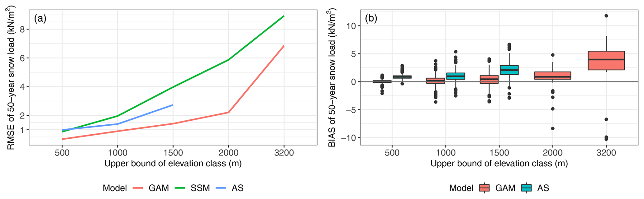
Figure 4RMSE (a) and bias (b) of 50-year snow loads for the different models and the Austrian standard (AS) classified by elevation. GAM stands for the generalized additive model, SSM for the smooth spatial model. The corresponding number of values within the elevation classes can be found in Fig. 2. Note that the current Austrian standard is not valid for elevations above 1500 m.
Figure 3 shows 50-year return levels of Δsnow-modeled yearly maxima locally fitted to a GEV distribution for all 897 stations as described in Sect. 2. More than 75 % of the values are below 4 kN m−2, with 50 % being smaller than 2.2 kN m−2, especially in the lower elevations in the north, east and southeast. As expected, the highest values occur in the snowy northern and southern Alps, where topography enhances precipitation. Only eight stations between 1740 and 3109 m exhibit a 50-year snow load return level larger than 15 kN m−2.
As outlined in Sect. 2.2 and explained in more detail in the Appendix, the best-suited GAM was found via a 10-fold cross-validation by fitting a GEV distribution to Δsnow-modeled maxima at the available 897 stations. In the notation of the R package mgcv (Wood, 2017) it is
Thereby ∼ signals a formula; “maxima”, “long”, “lat” and “alt” refer to yearly snow load maxima, longitude, latitude and altitude at a station; “s” marks an isotropic smoother with a thin plate regression spline as a basis function; and “k” defines the dimension of the basis function, i.e., the degrees of freedom available for this term. Note that a possible improvement of the suggested model would mean a significant effort, which is associated with increased hardware resources. To test the goodness of fit of the best GAM (Eq. 1) the Anderson–Darling test statistics were used as suggested by Le Roux et al. (2020). Using the R package gnFit Saeb (2018), the test was applied to quantiles retrieved from the distribution modeled with Eq. (1) to assess whether they are likely to follow a GEV distribution at the 5 % significance level. This is true for 88 % of all used stations.
The best SSM for comparison was found via an AIC-based model selection procedure, which led to the following model for the three GEV parameters (see Appendix for details):
Table 1 shows RMSE and bias of the GAM, SSM and the current Austrian snow load map (ASI, 2018) with respect to 50-year return values of Δsnow-modeled yearly maxima locally fitted to a GEV distribution. The scores for the GAM and SSM were obtained by a leave-one-out cross-validation with the models (Eqs. 1 and 2).
Table 1Error measures for 50-year return levels of snow load for the generalized additive model (GAM), smooth spatial model (SSM) and Austrian standard (AS), calculated using all 897 stations. (687 stations within Austria and below 1500 m for AS.) The scores are shifted in favor of the GAM if only stations within the Austrian border and below 1500 m are used. The RMSE value of the GAM is only 0.85 kN m−2 then (not shown).
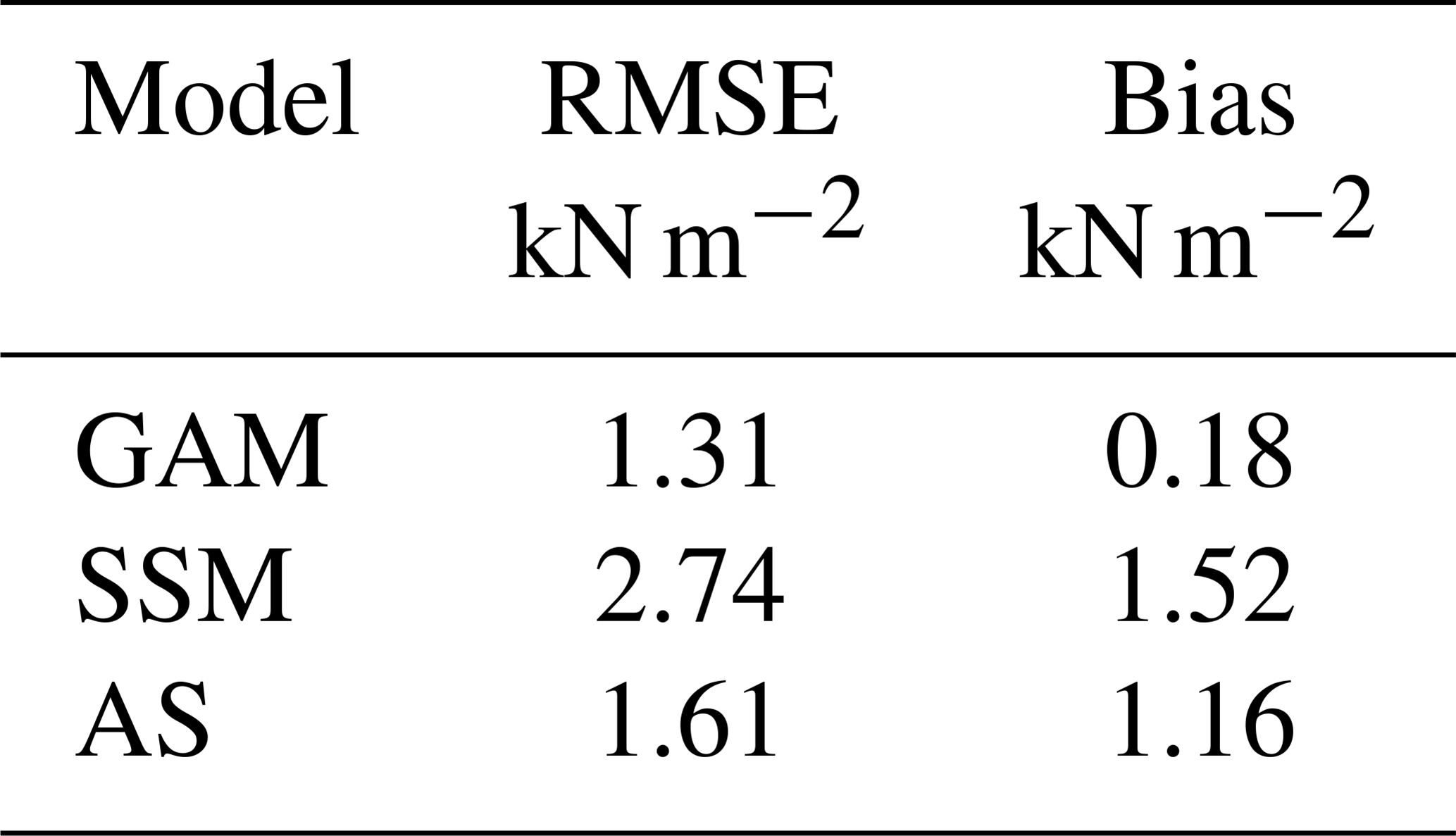
While both models and also the Austrian standard mostly overestimate reference snow loads, the GAM has the smallest RMSE and a very small, slightly positive bias. This is also confirmed in Fig. 4. Although the SSM uses more covariates, it is not able to model larger snow loads well. The GAM stays below an RMSE of 2.2 kN m−2 up to 2000 m and rises to 6.9 kN m−2 for elevations beyond 3000 m. This is accompanied by an increasing bias, which could at least partly be traced back to the small sample of only 14 stations in the highest elevation class (see Fig. 2). The newly proposed GAM approach shows smaller errors throughout all elevations when compared to the Austrian standard, even above 1500 m, but this must be considered with caution as the number of stations with elevations above 1500 m is only 57 (see Fig. 4).
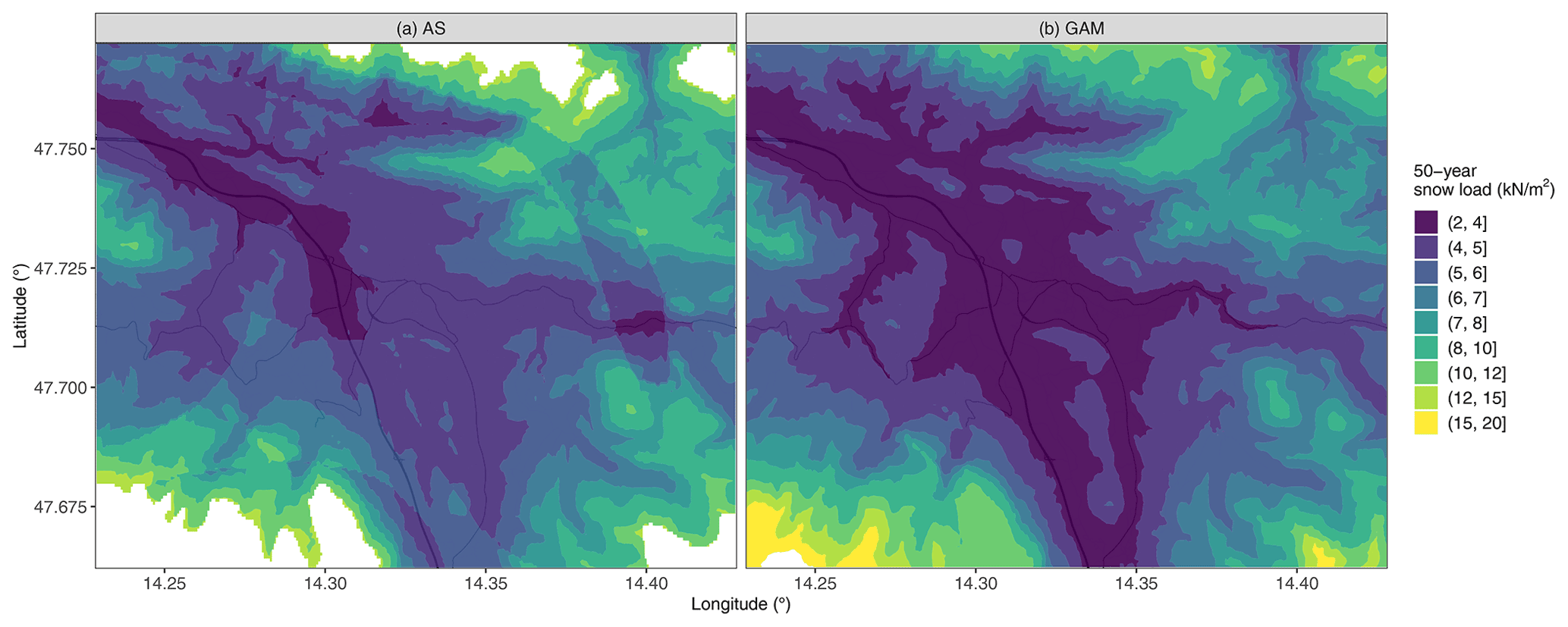
Figure 5Values of 50-year snow load return for a region around Windischgarsten in the center of Austria, taken from the map of the current Austrian snow load standard (a, AS; valid up to 1500 m) and the newly proposed GAM approach (b, plotted up to 2000 m). Pixel size is 50 m by 50 m. Main roads are depicted in the background for easier orientation.
The elevation class 1500 to 2000 m exhibits two severe negative outliers in the right panel of Fig. 4. Their locally estimated 50-year snow load return values are 14.1 and 15.2 kN m−2. Both stations are situated in very snowy regions at elevations of 1905 and 1740 m, respectively. Modeling snow loads smoothly in space eliminates another shortcoming of current standards. As outlined in the introduction, European snow load standards rely on zonings. This drawback is outlined in the left panel of Fig. 5, which shows a region in the center of Austria around the village of Windischgarsten. Several strangely curved features can be noticed, resulting from sudden transitions between zones. This leads to jumps of snow load values. Furthermore, the current Austrian standards only allow for calculating sk up to 1500 m elevation (white regions in the left panel of Fig. 5). The GAM approach (right panel in Fig. 5) is able to model smooth transitions while showing acceptable accuracy also at higher elevations (up to 2000 m in Fig. 5).
A transparent way towards a reproducible snow load map, conformable to CEN standards (CEN, 2015), is proposed: (i) simulating snow loads with the Δsnow model at intensively quality-checked, long-term snow depth records and (ii) using a generalized additive model (GAM) with penalized regression splines to spatially interpolate the generalized extreme value (GEV) distribution of the simulated snow load records. This procedure results in a map with smooth values of characteristic snow loads (sk).
The presented methodology is proposed for the successor of the current Austrian snow load standard (ASI, 2018). The potential of the two-stage Δsnow – GAM approach could be shown. The RMSE and bias with respect to 50-year snow load references at 897 stations are much smaller than for smooth modeling or the current standard. However, for very high elevations above 2000 m the error measures reach unacceptably large values. Only longitude, latitude and altitude were used as explaining covariates. This not only ensures relatively low model complexity but also keeps the application of the method easy.
A similar approach, combining the methods of snow load simulation and appropriate spatial extreme value modeling, could be applied in other countries as well since long-term snow records are the only prerequisite. This would minimize inconsistencies of snow load standards at national borders, a target expressed by the European Committee for Standardization (CEN, 2015). The proposed approach avoids zoning and mitigates altitudinal restrictions. It provides a base to update snow load maps to current climatic conditions as suggested by the coming Eurocode (CEN, 2020, Annex A.5). On this fundament, finally, efforts of implementing possible climate-change-related trends of snow load extremes (like Croce et al., 2018; Le Roux et al., 2020) could be built on for a future generation of snow load standards.
The R package mgcv (Wood, 2017) is used to fit a GEV spatially to snow load maxima. Smooth terms are represented by penalized regression splines, and the smoothing parameters are estimated during the fitting process. To find a suitable GAM for the spatial representation of snow load maxima, the following steps were performed: firstly a null model was defined in the notation of the R package mgcv, using the covariates longitude (long), latitude (lat) and altitude (alt):
Thereby “maxima” refers to yearly snow load maxima at a station, and the term “s” stands for a smooth term with a thin plate regression spline (Wood, 2003) as a basis function. Note that the intuitive standard, namely using one smooth term for each of the three covariates, leads to worse AIC and RMSE values. For the null model (Eq. A1), the dimension of the basis “k” is estimated during the fitting process. For the available 897 stations, the values were estimated to k=29 for the first term, s(long, lat), and k=9 for the second term, s(alt).
Secondly, the complexity of the GAM was incrementally increased for both terms by allowing more degrees of freedom, i.e., increasing k. Therefore the dimension k for the first term, s(long, lat), was set to 60, 120, 200 and 400 and in only one step to 20 for the second term, s(alt). The most complex model was then
To find the best suitable GAM and to avoid overfitting, a 10-fold cross-validation for each model was performed. The dataset of 897 stations was randomly split into 10 subsets (Fig. A1). In 10 passes, 9 subsets were always used as a training dataset and the remaining one as testing dataset.
Figure A2 shows the evolution of the RMSE and AIC for training and testing datasets calculated from the first five models and the locally estimated 50-year return levels of Δsnow-derived snow loads using maximum likelihood for parameter estimation. The more complex models with k=20 for the s(alt) term led to larger RMSE values for both the training and testing datasets and are not shown.
With increasing k, i.e., degrees of freedom, the RMSE of both the training and testing datasets always decreases. But for k>120 the testing dataset no longer benefits from increasing complexity, which is the point where overfitting sets in. As expected, the AIC also decreases (numbers in Fig. A2). Therefore a model (Eq. A1) with k=120 for the first term and k=9 for the second term was selected as the best GAM.
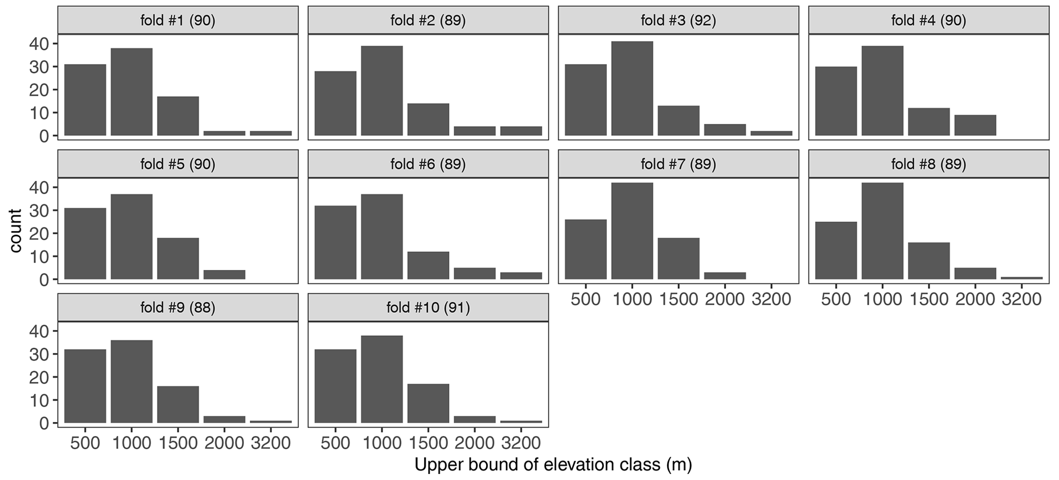
Figure A1Elevation histograms of the 10 randomly found subsets of all 897 stations. Respective number of members is given in brackets.

Figure A2Lines show the RMSE based on a 10-fold cross-validation of all 897 stations for testing and training datasets for models with increasing degrees of freedom. The numbers refer to the largest AIC of the training datasets out of 10 passes for each degree of freedom.
To fit a smooth spatial model (SSM) to the snow load maxima we followed the approach of Gstöhl (2017) as a blueprint. As covariates for the SSM, longitude, latitude and altitude are used, but the location and scale parameter are also allowed as explaining covariates. To select the best regression formula for each of the three GEV parameters, a generalized linear regression between the GEV parameter (e.g., μ) and covariates added stepwise was performed. The formula between a null model (e.g., μ∼1) and a given full model (e.g., location parameter μ ∼ all covariates) leading to the smallest AIC was selected.
R code used in this study is available from the authors upon reasonable request.
The observations used in this study are generally not freely available. However, in compliance with particular regulations they are available on request from ZAMG for research purposes.
HS and MW developed and designed the project together. HS did the coding and wrote the manuscript together with MW. MW raised the funding through his commitment at Austrian Standards International. TH helped with model development.
The authors declare that they have no conflict of interest.
Publisher's note: Copernicus Publications remains neutral with regard to jurisdictional claims in published maps and institutional affiliations.
This article is part of the special issue “Applied Meteorology and Climatology Proceedings 2020: contributions in the pandemic year”.
The framework for this paper was provided by the “Schneelast.Reform” project, managed by Ulrich Hübner from the Association of the Austrian Wood Industries (FV Holzindustrie) and supported by the Austrian Research Promotion Agency (FFG; grant nos. 870909 and 879303) and the Austrian Economic Chamber (WKO). The authors are thankful for this support. We also thank Alexander Radlherr and Susanne Drechsel (ZAMG, Austria) as well as Gilbert Kotzbeck (LFRZ, Austria) for their help with data and mapping, respectively. The Swiss SLF and the Hydrographic Service of Tyrol, Austria, are thanked for providing the snow data.
This research has been supported by the Österreichische Forschungsförderungsgesellschaft (grant nos. 870909 and 879303).
This paper was edited by Tanja Cegnar and reviewed by three anonymous referees.
Akaike, H.: A new look at the statistical model identification, IEEE T. Automat. Contr., 19, 716–723, https://doi.org/10.1109/TAC.1974.1100705, 1974. a
ASI: ÖNORM B 1991-1-3:2018 12 01, Austrian Standards Institute, Vienna, Austria, 2018. a, b, c, d, e
Auer, I., Böhm, R., Jurkovic, A., Lipa, W., Orlik, A., Potzmann, R., Schöner, W., Ungersböck, M., Matulla, C., Briffa, K., Jones, P., Efthymiadis, D., Brunetti, M., Nanni, T., Maugeri, M., Mercalli, L., Mestre, O., Moisselin, J.-M., Begert, M., Müller-Westermeier, G., Kveton, V., Bochnicek, O., Stastny, P., Lapin, M., Szalai, S., Szentimrey, T., Cegnar, T., Dolinar, M., Gajic-Capka, M., Zaninovic, K., Majstorovic, Z., and Nieplova, E.: HISTALP – historical instrumental climatological surface time series of the Greater Alpine Region, Int. J. Climatol., 27, 17–46, https://doi.org/10.1002/joc.1377, 2006. a
Autonome Provinz Bozen Südtirol: Dekret des Landeshauptmanns vom 6. Mai 2002, Nr. 14, available at: http://lexbrowser.provinz.bz.it/doc/de/dpgp-2002-14/dekret_des_landeshauptmanns_vom_6_mai_2002_nr_14 (last access date: 28 July 2021), 2002. a
Blanchet, J. and Lehning, M.: Mapping snow depth return levels: smooth spatial modeling versus station interpolation, Hydrol. Earth Syst. Sci., 14, 2527–2544, https://doi.org/10.5194/hess-14-2527-2010, 2010. a, b
CEN: EN 1991-1-3:2003/A1:2015, European Committee for Standardization, Brussels, Belgium, 2015. a, b, c, d, e, f, g, h
CEN: SC1.T2; N 1469; Final Draft EN 1991-1-3 “Snow Loads”, European Committee for Standardization, Brussels, Belgium, 2020. a, b, c, d
Coles, S.: An Introduction to Statistical Modeling of Extreme Values, in: Springer Series in Statistics, Springer-Verlag, London, https://doi.org/10.1007/978-1-4471-3675-0, 2001. a
Croce, P., Formichi, P., Landi, F., Mercogliano, P., Bucchignani, E., Dosio, A., and Dimova, S.: The snow load in Europe and the climate change, Clim. Risk Manage., 20, 138–154, https://doi.org/10.1016/j.crm.2018.03.001, 2018. a
Croce, P., Formichi, P., Landi, F., and Marsili, F.: Harmonized European ground snow load map: Analysis and comparison of national provisions, Cold Reg. Sci. Technol., 168, 102875, https://doi.org/10.1016/j.coldregions.2019.102875, 2019. a
DeBock, D. J., Liel, A. B., Harris, J. R., Ellingwood, B. R., and Torrents, J. M.: Reliability-Based Design Snow Loads. I: Site-Specific Probability Models for Ground Snow Loads, J. Struct. Eng., 143, 04017046, https://doi.org/10.1061/(ASCE)ST.1943-541X.0001731, 2017. a
DIN: DIN EN 1991-1-3/NA:2019-04, Deutsches Institut für Normung e.V., Berlin, Germany, 2019. a
Etienne, C., Lehmann, A., Goyette, S., Lopez-Moreno, J.-I., and Beniston, M.: Spatial Predictions of Extreme Wind Speeds over Switzerland Using Generalized Additive Models, J. Appl. Meteorol. Clim., 49, 1956–1970, https://doi.org/10.1175/2010JAMC2206.1, 2010. a
Gaume, J., Eckert, N., Chambon, G., Naaim, M., and Bel, L.: Mapping extreme snowfalls in the French Alps using max-stable processes, Water Resour. Res., 49, 1079–1098, https://doi.org/10.1002/wrcr.20083, 2013. a
Gstöhl, S.: Spatial modeling of extreme snow depth and snow water equivalent, MS thesis, University of Innsbruck, Innsbruck, 2017. a
Guyennon, N., Valt, M., Salerno, F., Petrangeli, A. B., and Romano, E.: Estimating the snow water equivalent from snow depth measurements in the Italian Alps, Cold Reg. Sci. Technol., 167, 102859, https://doi.org/10.1016/j.coldregions.2019.102859, 2019. a
Haan, L. D.: A Spectral Representation for Max-stable Processes, Ann. Probabil., 12, 1194–1204, https://doi.org/10.1214/aop/1176993148, 1984. a
Hastie, T. J. and Tibshirani, R. J.: Generalized Additive Models, CRC Press, London, 1990. a
Hong, H. P. and Ye, W.: Analysis of extreme ground snow loads for Canada using snow depth records, Nat. Hazards, 73, 355–371, https://doi.org/10.1007/s11069-014-1073-z, 2014. a
Jonas, T., Marty, C., and Magnusson, J.: Estimating the snow water equivalent from snow depth measurements in the Swiss Alps, J. Hydrol., 378, 161–167, https://doi.org/10.1016/j.jhydrol.2009.09.021, 2009. a
Lehning, M., Bartelt, P., Brown, B., Fierz, C., and Satyawali, P.: A physical SNOWPACK model for the Swiss Avalanche Warning Services. Part II: Snow Microstructure, Cold Reg. Sci. Technol., 35, 147–167, https://doi.org/10.1016/S0165-232X(02)00073-3, 2002. a
Le Roux, E., Evin, G., Eckert, N., Blanchet, J., and Morin, S.: Non-stationary extreme value analysis of ground snow loads in the French Alps: a comparison with building standards, Nat. Hazards Earth Syst. Sci., 20, 2961–2977, https://doi.org/10.5194/nhess-20-2961-2020, 2020. a, b, c, d
Marty, C. and Blanchet, J.: Long-term changes in annual maximum snow depth and snowfall in Switzerland based on extreme value statistics, Climatic Change, 111, 705–721, https://doi.org/10.1007/s10584-011-0159-9, 2012. a
Mo, H. M., Dai, L. Y., Fan, F., Che, T., and Hong, H. P.: Extreme snow hazard and ground snow load for China, Nat. Hazards, 84, 2095–2120, https://doi.org/10.1007/s11069-016-2536-1, 2016. a
Nicolet, G., Eckert, N., Morin, S., and Blanchet, J.: Assessing Climate Change Impact on the Spatial Dependence of Extreme Snow Depth Maxima in the French Alps, Water Resour. Res., 54, 7820–7840, https://doi.org/10.1029/2018WR022763, 2018. a
Olefs, M., Schöner, W., Suklitsch, M., Wittmann, C., Niedermoser, B., Neururer, A., and Wurzer, A.: SNOWGRID – A New Operational Snow Cover Model in Austria, in: International snow science workshop proceedings 2013, Grenoble – Chamonix Mont Blanc, France, 38–45, available at: https://arc.lib.montana.edu/snow-science/item/1785 (last access: 28 July 2021), 2013. a
Olefs, M., Girstmair, A., Hiebl, J., Koch, R., and Schöner, W.: An area-wide snow climatology for Austria since 1961 based on newly available daily precipitation and air temperature grids, in: Geophysical Research Abstracts, vol. 19, EGU, Vienna, Austria, EGU2017–12249, 2017. a
ON: ÖNORM B 4013:1983 12 01, Österreichisches Normungsinstitut, Vienna, Austria, 1983. a
ON: ÖNORM B 1991-1-3:2006 04 01, Österreichisches Normungsinstitut, Vienna, Austria, 2006. a
Perčec Tadić, M., Zaninović, K., and Sokol Jurković, R.: Mapping of maximum snow load values for the 50-year return period for Croatia, Spat. Statist., 14, 53–69, https://doi.org/10.1016/j.spasta.2015.05.002, 2015. a
Saeb, A.: gnFit: Goodness of Fit Test for Continuous Distribution Functions, r package version 0.2.0, available at: https://CRAN.R-project.org/package=gnFit (last access: 28 July 2021), 2018. a
Sanpaolesi, L., Currie, D., Sims, P., Sacré, C., Stiefel, U., Lozza, S., Eiselt, B., Peckham, R., Solomos, G., Holand, I., Sandvik, R., Gränzer, M., König, G., Sukhov, D., del Corso, R., and Formichi, P.: Scientific support activity in the field of structural stability of civil engeneering works – snow loads, Final Report I Contract no. 500269 dated 16 December 1996, Commission of the European communities GDIII – D3, available at: http://www2.ing.unipi.it/dic/snowloads (last access: 28 July 2021), 1998. a, b
Sanpaolesi, L., Brettle, M., Currie, D., Dillon, P., Sims, P., Delpech, P., Dufresne, M., Sacré, C., Stiefel, U., Lozza, S., Eiselt, B., Peckham, R., Solomos, G., Holand, I., Leira, B., Sandvik, R., Gränzer, M., König, G., Sukhov, D., del Corso, R., and Formichi, P.: Scientific support activity in the field of structural stability of civil engeneering works – snow loads, Final Report II Contract no. 500990 dated 12 December 1997, Commission of the European communities GDIII – D3, available at: http://www2.ing.unipi.it/dic/snowloads (last access: 28 July 2021), 1999. a
Schellander, H. and Hell, T.: Modeling snow depth extremes in Austria, Nat. Hazards, 94, 1367–1389, https://doi.org/10.1007/s11069-018-3481-y, 2018. a, b, c, d, e, f
Schellander, H. and Winkler, M.: niXmass – R package, available at: https://CRAN.R-project.org/package=nixmass (last access: 28 July 2021), 2020. a
Sezer, A., Kan Kilinc, B., and Yazici, B.: Modeling extreme rainfalls using generalized additive models for location, scale and shape parameters, Appl. Ecol. Environ. Res., 14, 635–644, 2016. a
SIA: SIA 261:2020, Schweizerischer Ingenieur- und Architektenverein, Zurich, Switzerland, 2020. a
Sturm, M., Taras, B., Liston, G. E., Derksen, C., Jonas, T., and Lea, J.: Estimating Snow Water Equivalent Using Snow Depth Data and Climate Classes, J. Hydrometeorol., 11, 1380–1394, https://doi.org/10.1175/2010JHM1202.1, 2010. a
Unterstrasser, S. and Zängl, G.: Cooling by melting precipitation in Alpine valleys: An idealized numerical modelling study, Q. J. Roy. Meteorol. Soc., 132, 1489–1508, https://doi.org/10.1256/qj.05.158, 2006. a
Vionnet, V., Brun, E., Morin, S., Boone, A., Faroux, S., Le Moigne, P., Martin, E., and Willemet, J. M.: The detailed snowpack scheme Crocus and its implementation in SURFEX v7.2, Geosci. Model Dev., 5, 773–791, https://doi.org/10.5194/gmd-5-773-2012, 2012. a
Wastl, C. and Zängl, G.: Mountain–valley precipitation differences in the northern Alps: an exemplary high-resolution modeling study, Meteorol. Atmos. Phys., 108, 29–42, https://doi.org/10.1007/s00703-010-0083-y, 2010. a
Winkler, M., Kaufmann, H., Schöner, W., and Kuhn, M.: Schnee- und Eislast, in: ExtremA 2019, Aktueller Wissensstand zu Extremereignissen alpiner Naturgefahren in Österreich, Vienna University Press, Vienna, 2020. a
Winkler, M., Schellander, H., and Gruber, S.: Snow water equivalents exclusively from snow depths and their temporal changes: the Δsnow model, Hydrol. Earth Syst. Sci., 25, 1165–1187, https://doi.org/10.5194/hess-25-1165-2021, 2021a. a, b, c, d, e, f, g
Winkler, M., Schellander, H., Hübner, U., Radlherr, A., and Drechsel, S.: Schneelast.Reform, Endbericht, ZAMG – Zentralanstalt für Meteorologie Geodynamik, Innsbruck, Austria, in preparation, 2021b. a
Wood, S. N.: Thin plate regression splines, J. Roy. Stat. Soc. Ser. B, 65, 95–114, https://doi.org/10.1111/1467-9868.00374, 2003. a
Wood, S. N.: Generalized Additive Models: An Introduction with R, 2nd Edn., Chapman and Hall/CRC, Boca Raton, 2017. a, b
- Abstract
- Introduction
- Data and methods
- Results
- Conclusions and outlook
- Appendix A: Model selection for the generalized additive model
- Appendix B: Model selection for the smooth spatial model
- Code availability
- Data availability
- Author contributions
- Competing interests
- Disclaimer
- Special issue statement
- Acknowledgements
- Financial support
- Review statement
- References