Addressing up-scaling methodologies for convection-permitting EPSs using statistical and machine learning tools

Convection-permitting weather forecasting models allow for prediction of rainfall events with increasing levels of detail. However, the high resolutions used can create problems and introduce the so-called “double penalty” problem when attempting to verify the forecast accuracy. Post-processing within an ensemble prediction system can help to overcome these issues. In this paper, two new up-scaling algorithms based on Machine Learning and Statistical approaches are proposed and tested. The aim of these tools is to enhance the skill and value of the forecasts and to provide a better tool for forecasters to predict severe weather.

1 Introduction

Since the dawn of Numerical Weather Prediction (NWP), the increasing need for accurate prediction has grown as fast as advances in technology and modern high-performance computing (Bauer et al., 2015). Increasingly accurate forecasting of rainfall is required, particularly in the case of high-impact events where damages can run into the hundreds of millions of euro (Llasat et al., 2010). Operational convection-permitting models are now capable of forecasting such events at kilometre-scale resolutions; for a review, see Clark et al. (2016). However, the benefits of increased resolution are not always clear (Mass et al., 2002). The use and verification of high-resolution point forecasts of rainfall suffers from the so-called “double penalty” issue (Mittermaier, 2014). Convection-permitting models create a better spatial definition of precipitation structures compared to coarser resolution models and thus a shift in the precipitation pattern can occur when comparing model output with observations: when computing verification scores the model is punished twice as rain is predicted at an incorrect location and not predicted at the correct location.

As outlined in Palmer (2019) when forecasting on short temporal scales a probabilistic approach using an Ensemble Prediction System (EPS) is essential in order to deal with the inherently chaotic nature of the Earth's atmosphere. An EPS can also help overcome some of the deficiencies of a single deterministic forecast, including the double penalty problem for rainfall forecasts (Mittermaier, 2014).

One common post-processing approach for EPS forecasts is to use a neighbourhood processing technique called up-scaling (Clark et al., 2016; Ben Bouallègue and Theis, 2014; Marsigli et al., 2008). These works among others, e.g. (Duc et al., 2013), have demonstrated that using neighbourhood post-processing techniques give more skilful EPS forecasts. In the following, some simple neighbourhood up-scaling methods are investigated, as well as more complex machine learning algorithms. The goal is improved probabilistic forecasts, both in terms of addressing the double penalty of verification and, most importantly, in providing accurate products to operational forecasters. However, this paper focuses more on the details of the machine learning algorithms and the steps needed to implement each one rather than operational products.

Machine learning, as well as deep learning algorithms and neural networks are becoming increasingly popular and widespread throughout the scientific world for their natural quality of self-adjustment and self-learning (Bremnes, 2019; Grönquist et al., 2021). It is likely that such algorithms will find more and more applications in NWP (Dueben and Bauer, 2018). Tree-based ensemble methods have recently been successfully applied to improve the skill of low visibility conditions in an operational meso-scale model (Bari and Ouagabi, 2020), while Krasnopolsky and Lin (2012) demonstrated how machine learning algorithms can decrease the bias for low and high rainfall.

In this paper, up-scaling methods will be applied to a number of rainfall cases, using forecasts from the operational ensemble system in use at Met Éireann, the Irish national meteorological service. This system, along with the cases and observational data, will be introduced in Sect. 2, with the up-scaling techniques described in Sect. 3. Results from the test cases are presented in Sect. 4, followed by conclusions in Sect. 5.

2 Data and Test Cases

2.1 IREPS

The Irish Regional Ensemble Prediction System (IREPS) used for daily operations at Met Éireann is based on the system described in Frogner et al. (2019). IREPS uses the nonhydrostatic mesoscale HARMONIE-AROME canonical model configuration of the shared ALADIN-HIRLAM system (Bengtsson et al., 2017). IREPS currently consists of 1 control plus 10 perturbed members. The horizontal resolution used is 2.5 km, with a regional domain consisting of 1000×900 gridpoints in the horizontal, and 65 vertical levels; this domain is shown in Fig. 1. The operational cycling consists of 54 h forecasts four times daily (at 00:00, 06:00, 12:00 and 18:00 Z). Details of the various perturbations, physics and dynamics options used in IREPS and HARMONIE-AROME can be found in Frogner et al. (2019) and Bengtsson et al. (2017) respectively.

The test cases introduced below and reported on later in the paper's results focus on the rainfall forecast by IREPS in the 24 h from the 00:00 Z cycle. In order to reduce data sizes a domain cut-out over the island of Ireland was used (see Fig. 1).

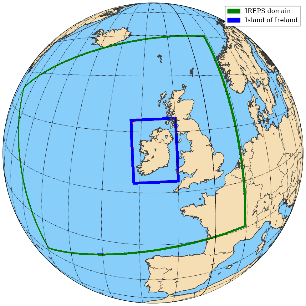
Figure 1 The operational IREPS domain (green) with the “Island of Ireland” sub-domain used in this study (blue).

2.1.1 9 of May 2020

This case study was exploited during the initial testing of the statistical and machine learning tools. It concerns an episode of strong convective activity over south-west Ireland on the 9 May 2020. The IREPS forecast reveals a rapid development of convective phenomena over the south-west of Ireland starting from hour 13:00 Z. Shown in Fig. 2 is a sample of the 00:00 Z forecast from the 9 May, along with radar observations. It can be seen that IREPS succeeded in capturing the main areas of rainfall but that some discrepancies existed in terms of the location of individual convective cells. Therefore, this case was deemed an appropriate event upon which to perform initial testing of the proposed algorithms.

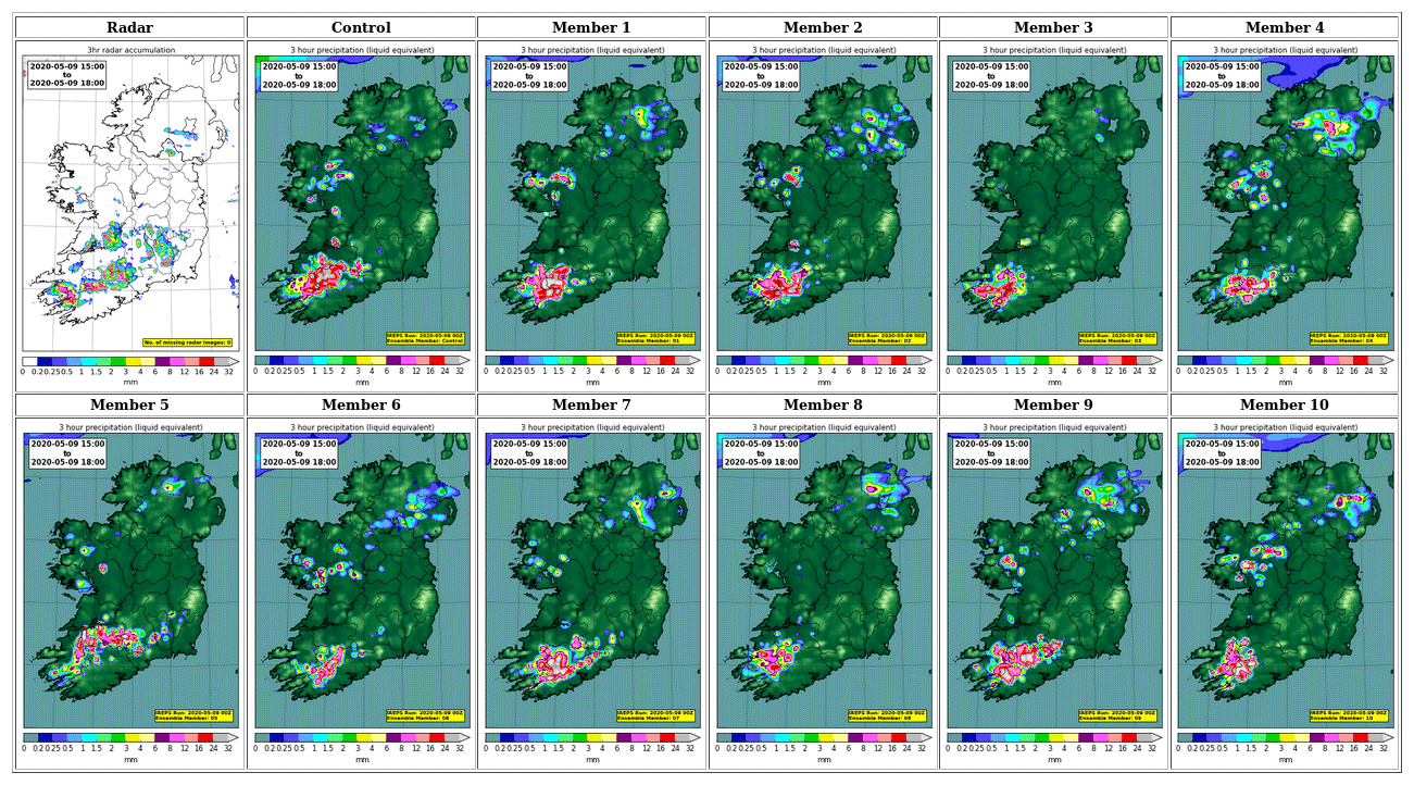
Figure 2 Three-hour rainfall accumulations from 15:00–18:00 Z on the 9 May 2020, when convective rainfall was triggered particularly in the south-west and south-east of the country. The top left panel shows observed accumulations from Met Éireann's operational radar. The remaining panels show the predicted amounts from the 11 members of the 00:00 Z IREPS cyle on the 9 May.

2.1.2 June 2020

June 2020 presented a rich variety of meteorological scenarios in terms of rainfall. Eight 24 h periods from June 2020 were investigated. A short description of the rainfall characteristics of the period is given in Table 1. The aim here is not to fully describe the meteorological details of each case but to give an idea of the rainfall field in the 00:00 Z cycle from IREPS for a given period. This June 2020 IREPS data serves as the dataset for the various algorithms in the discussion and results (Sect. 4).

2.2 Observations and verification metrics

The verification metrics in Sect. 4 make use of observations of 24 h accumulated rainfall recorded by synoptic and climate stations from Met Éireann's operational network (shown in Fig. 3). When matching forecasts to observations, the nearest IREPS grid-point to the observation station location was used. The Brier Score (BS), Relative Operating Characteristic (ROC) curve and Area Under the ROC (AUC) curve were the verification metrics of choice. A description of these scores can be found in Wilks (2011).

Table 1 Concise description of the 24 h rainfall forecasts from the 00:00 Z cycles of IREPS on the selected days in June 2020.

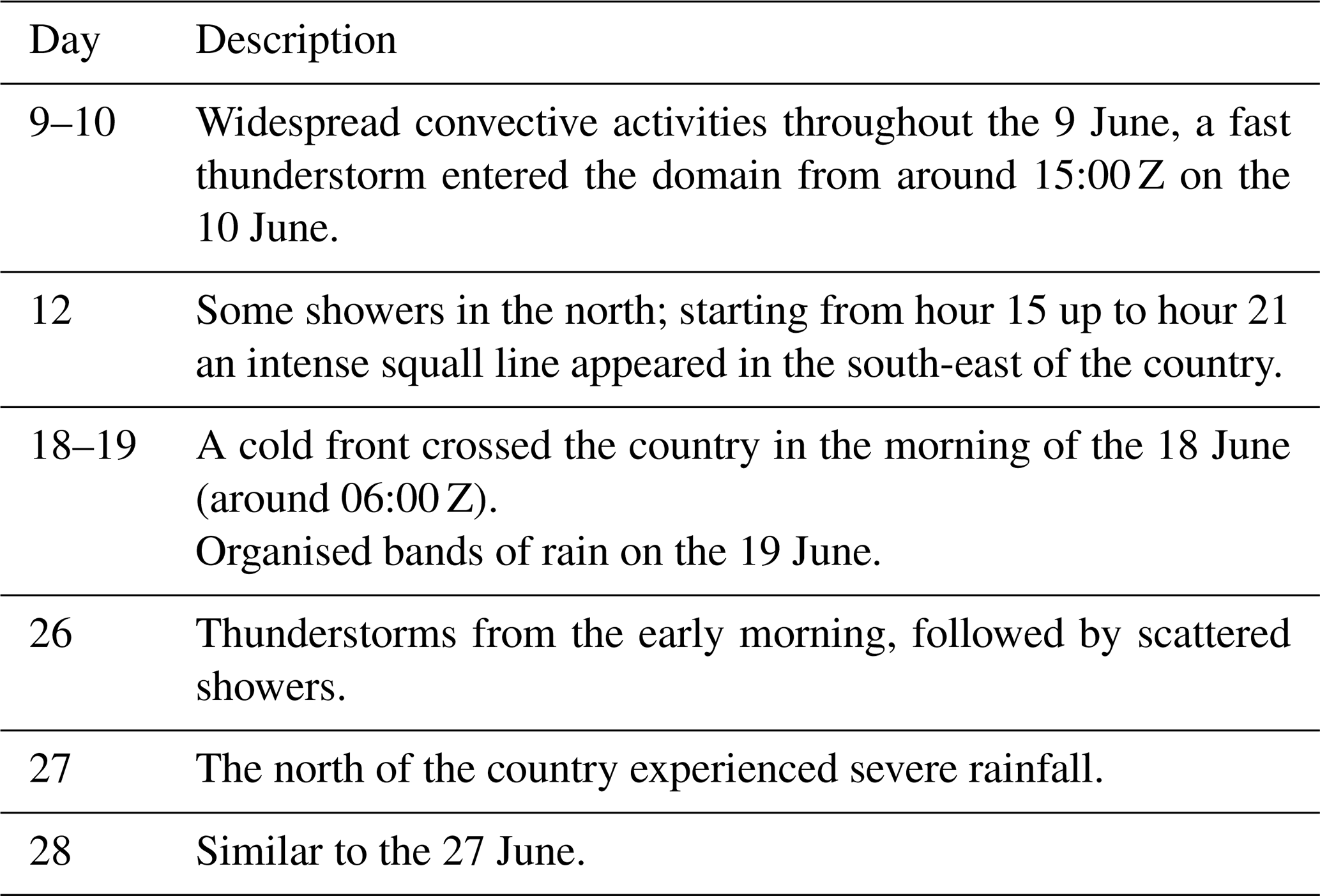
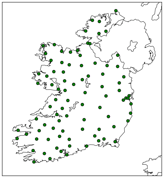
Figure 3 Met Éireann synoptic and automatic climate stations used.

3 Methodologies

In this section, different up-scaling methodologies are presented. The idea behind neighbourhood up-scaling is to reduce the double-penalty error by substituting each grid point with a reweighting that takes into account the forecasts at a number of neighbouring points (Ebert, 2008). The number of points used as a radius to define this neighbourhood may be fixed, in the simplest approach, or vary with meteorological conditions.

The up-scaling procedure may be neatly described by a matrix convolution as follows. Let M be a matrix associated with a two-dimensional rainfall field: either threshold exceedances or the ensemble probability of exceedance (further explanations are given in Sect. 3.1). Then the up-scaled field is given by

$$\begin{array}{}\text{(1)}& (\mathbf{M}*\mathbf{K})[i,j]=\sum _{n=\mathrm{1}}^L\sum _{l=\mathrm{1}}^L\mathbf{M}[i-n,j-l]\mathbf{K}[n,l]\end{array}$$

Here K is a square kernel matrix of dimension $L=(\mathrm{2}R+\mathrm{1})$, where R is the radius for the neighbourhood in the up-scaling, and indices in square brackets represent matrix entries. In the following subsections, three different methodologies are addressed: in Sect. 3.1 radius is kept constant over the entire domain, in Sect. 3.2 the kernel involved in the convolution changes based on the ensemble spread in the forecast, while in Sect. 3.3 the field is divided into groups and a specific R is assigned to up-scale each of them.

It should be noted that each algorithm returns a two dimensional array smaller than the input one because it takes into account enough distance from the borders to perform the convolution. The matrix covers a sub-section of the entire IREPS domain thus, points at the edge are treated alike without need of further manipulation.

3.1 Fixed Up-scaling

This subsection describes the basic up-scaling post-processing currently used by Met Éireann, which aims to better classify the occurrence of rain in a region rather than by expecting a perfectly precise geographic match. A fraction-like matrix is defined, here called the Fraction Probability Matrix (FPM). It is obtained as follows. First, the original precipitation field is mapped onto a Boolean form, allocating a logical value of 1 if the precipitation pr_ij is above a given threshold (e.g. th =5 mm) and 0 otherwise.

$$\begin{array}{}\text{(2)}& \mathbf{M}[i,j]=\left\{\begin{array}{l}\mathrm{1},{\mathrm{pr}}_{ij}\ge \mathrm{th}\\ \mathrm{0},{\mathrm{pr}}_{ij}<\mathrm{th}\end{array}\right.\end{array}$$

There are two main way to proceed at this stage. The convolution could be applied on each binary matrix followed by a summation. This approach requires some further manipulation, whereby a clipping function has to be applied to restrain values above the probabilistic range. However, there are a few disadvantages that must be taken into account. If working with an EPS with higher number of members (greater then N=11) this entire procedure becomes time-consuming. Additionally, the Boolean values retrieved after clipping assume a rain event even if only one member predicted it, which could cause over-counting.

Hence, a second approach is more convenient, in which a simple averaging is first applied before the up-scaling procedure is performed. This average defines the FPM as

$$\begin{array}{}\text{(3)}& \mathrm{FPM}={\displaystyle \frac{\mathrm{1}}{N}}\sum _{d=\mathrm{1}}^N{\mathbf{M}}_d\end{array}$$

where d is the index of the summation and N the number of available members. FPM has a probabilistic meaning. Indeed, the more members agree on rainfall occurrence, the likelier it is that the event will take place. The convolution from Eq. (1) is then applied to this matrix, using a square, uniform kernel made of ones, which span the entire domain. The value of the radius is typically R=2 (fixed). It is not feasible to expect to find a unique shape or dimension for K that will always return the best result for any meteorological scenario. Nevertheless, it is possible building up on this basic approach to increase performances of the post-process. In this spirit two alternatives are proposed.

3.2 Dynamical approach

Any up-scaling technique should ideally have a dynamical configuration in order to effectively adapt itself to extreme highly variable situations. The following approach endeavours to model the in-homogeneity of the rainfall distribution and seeks to recognise those regions where changes takes place. Areas at equal values of fraction probability are up-scaled by the same kernel, while a gradient highlights an edge between zones at different level of agreement within members which makes the radius settings more delicate. Thus, it is reasonable to assume that the value of R should change with respect to the value of spread around a point.

Variability is evaluated by an indicator. Among several metrics available, standard deviation is chosen as it is widely used to return the dispersion from the mean within a group of numbers (Wilks, 2011). In this sense, the algorithm aims to keep track of point-wise mutability. The algorithm can be summarised in the following steps, and these are illustrated in the flowchart in Fig. 9:

1. A window of odd size dimension is defined, within which the spread metric is going to be calculated (lets call it B). B has to be fixed and satisfy a few conditions: it should be much smaller than the actual size of the domain and greater than or equal to the biggest kernel accessible. For example, a square of 11 × 11 fits our request for the 216 × 152 matrix being studied (corresponding to the island of Ireland domain) with $max\left(R\right)=\mathrm{5}$.

2. A double nested loop running over rows and column allows to select each point of the FPM, which becomes the center of the pre-set B. The spread associated is calculated, taking into consideration every element within the square B. Note that the spread highlights the area of change and those points are the ones where the double penalty is usually worst.

3. Up-scaling is performed, using a Gaussian kernel (further details can be found in Appendix A) whose radius R will strictly depend on the spread value.

Implementation requires setting appropriate ranges of standard deviation and related radii. The list of radii is given as an input argument, while the standard deviation ranges are fixed. In such a way all possible configurations can be analysed, a total of n^k for n possible radii and k ranges. Undoubtedly, the number of parameters to be set is greatly increased compared to the fixed method, but the algorithm does offer flexibility. Tests with specific conditions were carried out to determine the most appropriate settings: in a situation when the EPS members are in agreement and the spread is low, the atmosphere is in a predictable state and a large radius would most likely not add great value to the forecast. On the other-hand, if spread is high then a medium or large radius should guarantee that an appropriate up-scaling is applied. The spread matrix in Fig. 4 gives an indication of the agreement between members for the 9 May test case. Note that it does not indicate if IREPS members concur in rainfall occurrence, but whether there is a change in the level of consistency.

Figure 5 displays how the performance differs between fixed and dynamical up-scaling. It is noteworthy that the greater differences are localised in regions of high spread, meaning that up-scaling performances are more relevant in those areas. Looking carefully at the picture on the left panel in Fig. 5 it is possible to observe that the up-scaling procedure has a sort of blurring and smoothing effect. The high-resolution properties are in fact scaled-up to a coarser level, which is translated into an attempt to not miss any convection.

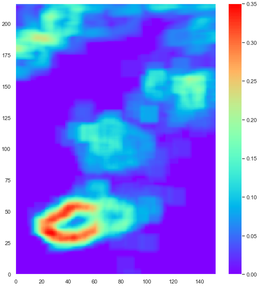
Figure 4 Spread matrix for the 9 May test case, constructed by replacing each point of the domain with the respective value of standard deviation.

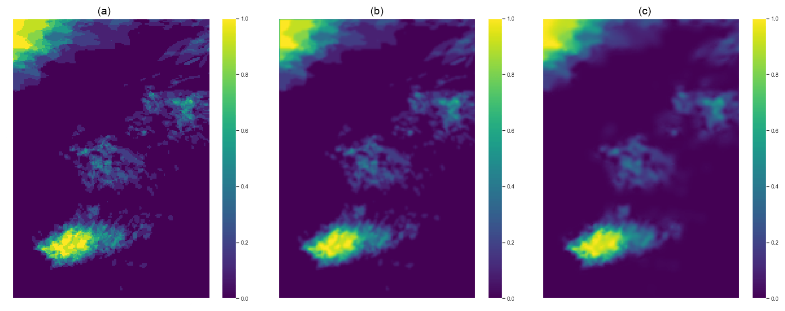
Figure 5 These three images allow for a qualitative comparison between the unupscaled FPM (a), the neighbourhood approach with fixed radius R=2 (b), and the spread based algorithm (c). The precipitation threshold is set to th =2 mm.

3.3 Hierarchical clustering based technique

A second up-scaling approach is now proposed based on a machine learning tool in which a pattern recognition ability is employed, i.e. the capability of arranging data or information in regular and well defined structures. Further information on the underlying strategy can be found in Bonaccorso (2019). The major assumption for the current technique is that the radius choice can be based on clustering, discriminating kernel dimensions with respect to the level of cluster aggregation. Hence, elements aggregated within the same group should be up-scaled in the same way using a common radius. Most unsupervised (as well as supervised) machine learning techniques have the major disadvantage of requiring the number of clusters to be defined a priori. This is an arbitrary hyperparameter, whose choice is usually made by data diagnostics or feature graphical analysis. However, such an approach is impractical in NWP as it would mean going through every daily forecast product manually. Thus, it must be provided by the code itself and so the core scheme employed here is the Hierarchical clustering algorithm, with which it is possible to automate the number of clusters.

A Hierarchical aggregation framework treats all objects in a given initial set as an individual group and by step-wise comparison it progressively discovers the best way to group them together based on similarity level. All elements are jointly exhaustive (each point must be in one subset) and mutually exclusive (the same point can not be found in more than one subset). Data are stored into column arrays with which the algorithm is fed. Then, the Hierarchical clustering starts analysing every observation as a cluster and after each iteration two groups (containing one or more observations) are gathered. When all remaining elements are aggregated in one single cluster the algorithm stops. Specifications regarding the step-wise aggregation are chosen as follow: similarity between grid values (inner-elements distance) is estimated using a standard L² norm, while a single linkage criterion establishes inner-group proximity; see, again, Bonaccorso (2019) for details.

A first testing phase was conducted on the case-study described in Sect. 2.1.1 in order to determine whether or not hierarchical aggregation is able to correctly capture pattern structure in our datasets. Three main features were considered: latitude, longitude and rainfall (note that the up-scaling algorithm here described makes use of the FPM as input, but a first check was made on the precipitation field).

From a meteorological perspective, latitude and longitude are less relevant, given the small scale of Ireland, although topography is certainly relevant to a convective rainfall field at the boundary and could be interesting to explore. It can be seen in the right panel of Fig. 6, latitude and longitude coordinates seem to mislead the algorithm, taking over as the most important properties. In general, features could be re-scaled with some normalisation. However, it is here possible to achieve a good clustering by neglecting latitude and longitude, forcing the algorithm to work with the accumulated precipitation data only. Qualitative plots verifying the desired ability of aggregation recognition can be found in Fig. 6.

In a similar manner to the dynamical approach in Sect. 3.2, a flowchart for the algorithm is presented in Fig. 9, with the main steps explained in more details as follows:

1. As previously mentioned, Hierarchical clustering requires one-dimensional arrays. Therefore, the FPM is reshaped from 2D matrix to a column value arrangement. In such a way it can be treated as a feature by the linkage operation.

2. The number of clusters is obtained via a dendrogram, a graphical representation of the cumulative hierarchical progression to display relationships of data. A dendrogram is a tree-like plot, where data are listed along the x-axis by an index label and values of similarity derived from the linkage on the y-axis. Chen et al. (2009) investigate further usage of this tool for large dataset. A limit line is traced between two steps, where there is the highest rise in similarity (implying the greater dissimilarity from the previous aggregation and the next one). The dendrogram's branches are crossed a number of times by the horizontal bar. This is the adequate hyperparameter to be used.

3. Once the number of cluster is established, each grid-point has to be associated to a group. Therefore, the agglomerative clustering is performed to get aggregation prediction. When dealing with the FPM, points having similar fraction probability are grouped together as is shown in Fig. 7.

4. Each point within a cluster is up-scaled using the usual convolution operation and the assigned radius. A further scaling is required to maintain values in the range [0,1].

An example of the up-scaled output from this algorithm is shown in Fig. 8.

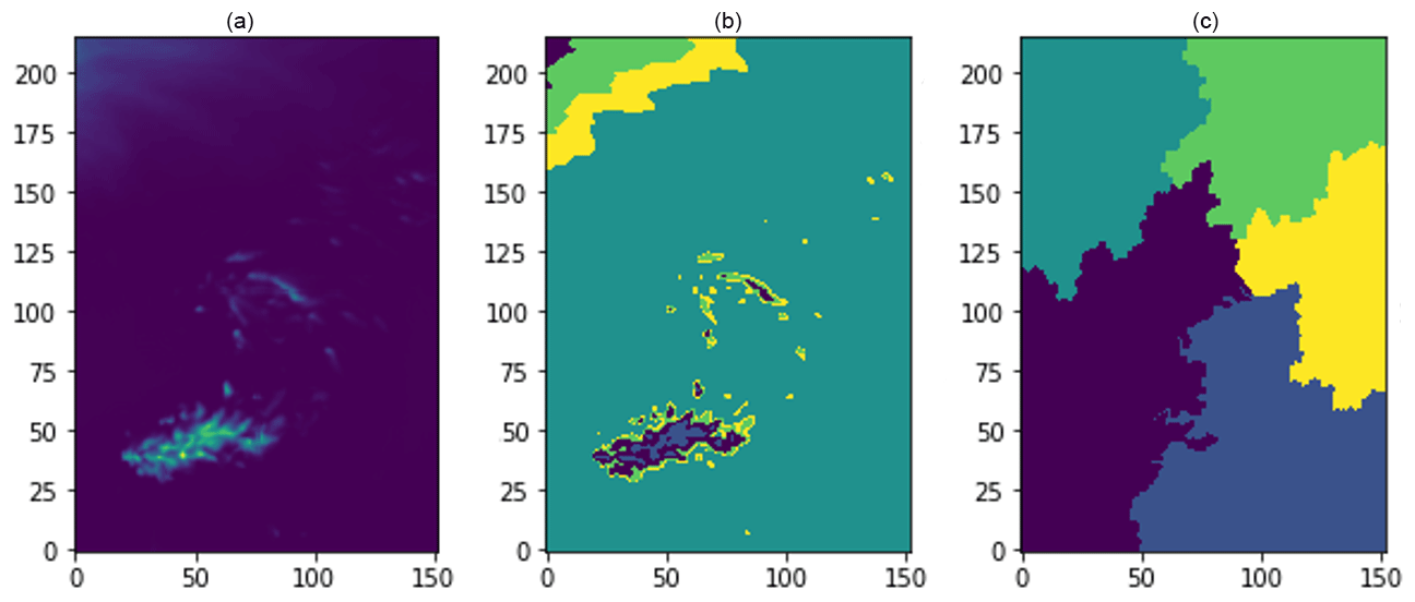
Figure 6 On the left side of the panel, a snapshot of the total rainfall field forecast at +24 h for the 9 May 2020 is displayed. The right image shows the hierarchical aggregation's attempt to use all the features (latitude, longitude and rainfall). The central plot displays the cluster pattern achieved using accumulated rainfall as the unique attribute.

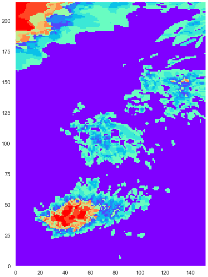
Figure 7 Result from step 3 of the hierarchical clustering algorithm. The aggregation prediction associates each point of the domain with one cluster. Each color represents a cluster.

Figure 8 Clustering based up-scaling, with a combination of $R=\mathit{\{}\mathrm{2},\mathrm{3},\mathrm{4},\mathrm{5},\mathrm{6}.\mathit{\}}$ and th =2 mm.

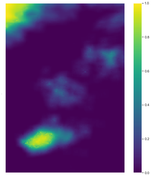
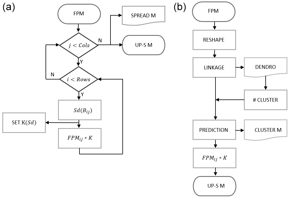
Figure 9 Flowchart representation of the schemes of action for the spread-base up-scaling (a) and the clustering-based one (b). Further description and details of the terminology may be found in the text.

4 Discussion and Results

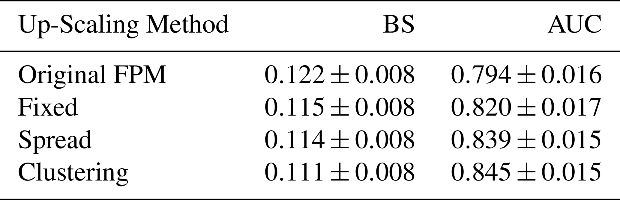
Table 2 details the BS and AUC scores for 24 h rainfall forecasts for the IREPS 9 May and June 2020 datasets. The skill score values represent the mean values for all methodologies described in Sect. 3; “Original FPM” refers to the method described to map the source data of rainfall onto the FPM using Eqs. (2) and (3), “Fixed” in Sect. 3.1, “Spread” in Sect. 3.2 and “Clustering” in Sect. 3.3.

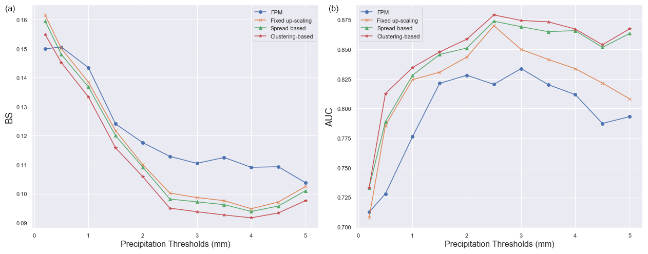
The precipitation thresholds [0.2, 0.5 and 1.0–5.0 mm in 0.5 mm increments] were chosen so as to ensure usable statistics from each of the days in the dataset. This gives in total a sample size of 11 thresholds over the nine 24 h periods. Statistics are calculated over the island of Ireland domain illustarted in blue in Fig. 1.

As illustrated by both the BS and AUC scores, the machine learning based clustering approach gives the most satisfactory results, with a mean BS of 0.111 and an AUC of 0.845. The improvement in AUC score in particular between the “Original FPM” method and the “Clustering” method is noteworthy. This suggests that IREPS rainfall forecasts could benefit from a post-processing technique based on a clustering technique. The “Fixed”, “Spread” and “Clustering” methodologies all illustrate improvements over the “Original FPM”.

Figures 10 display a series of skill score values for the 24 h rainfall thresholds detailed above. Both the BS and AUC scores in Fig. 10 demonstrate the superiority of the “Clustering” based approach for all thresholds (except for the BS 0.1 mm threshold where the “Original FPM” performs slightly better). Both time series indicate a hierarchy of performance; the “Spread” and “Fixed” approaches being slightly less skilful than the “Clustering” but clearly out-performing the “Original FPM”. From the BS time series, the increase in skill is most evident for the thresholds above 1.5 mm.

The improvement in both BS and AUC scores for each of the up-scaling techniques is encouraging. The results clearly demonstrate the need for the up-scaling of EPS convective rainfall forecasts, as has been reported by many others (Mittermaier, 2014; Osinski and Bouttier, 2018).

It is important to note that these results aim to show a general improvement in the post-processed skill scores by the various statistical and machine learning algorithms, not to prove their supremacy in all scenarios. Indeed there are some scenarios where the basic fixed up-scaling performs better (not shown). The BS and AUC scores presented here were calculated using synoptic and climate stations. A more thorough and robust verification of the various algorithms could be performed by calculating skill scores using radar data to ensure better spatial coverage and a greater sample size. It must also be noted that the advantage of the “Spread” and “Clustering” methodologies is that the control parameters of each method can be modified in order to reach a better verification score.

Table 2 Mean value of BS and AUC calculated for 9 May and case studies in Table 1 at +24hour, and for the following set of thresholds: $\mathit{\{}\mathrm{0.2},\mathrm{0.5},\mathrm{1.0},\mathrm{1.5},\mathrm{2.0},\mathrm{2.5},\mathrm{3.0},\mathrm{3.5},\mathrm{4.0},\mathrm{4.5},\mathrm{5.0}\mathit{\}}$ mm. The associated error is calculated as Standard Error of the Mean (SEM).

Figure 10 Brier Score (a) and Area Under the ROC Curve (AUC) skill scores (b) with respect to rainfall threshold for 24 h IREPS forecasts for 9 May and June days presented in Table 1. The lines represent the methodologies outlined in Sect. 3.

5 Conclusions

The role of post-processing is undoubtedly fundamental to issues affecting NWP products, which still use approximated theories or parametrizations to reproduce behaviours at small spatial scales that NWP model resolutions cannot handle.

In this paper, two neighbourhood approaches for convective-permitting models based on a statistical post-processing and a machine learning technique were proposed. Objective verification results demonstrated that the machine learning approach gave an improvement over more traditional up-scaling approaches.

A number of aspects were not explored in this work however. A more robust dataset with a more diverse set of meteorological scenarios would need to be investigated in order to make concrete statements about the supremacy of the machine learning technique.

Furthermore, the dependency on the weather scenario should be taken into account and so a deeper exploratory analysis is required in order to set all arbitrary hyper-parameters in the chosen algorithms to adapt along with an evolution in weather patterns. Other machine learning techniques, e.g. convolutional neural networks (Bremnes, 2019) could also be explored. Early work on the implementation of a methodology based on a combination of both the clustering and spread up-scaling has begun. This approach aims to take advantage of the strengths of both methods.

The results described here have focused solely on convective rainfall in the summer period. Testing the methodologies on rainfall episodes during Ireland's winter may uncover a preference for other methodologies, as could an investigation into the up-scaling of other meteorological variables (e.g. 10 m wind speed, 2 m temperature). Finally, a more global solution could be to base the choice of up-scaling algorithm on the atmosphere's large-scale dynamics (Allen and Ferro, 2019).

Appendix A: Gaussian Kernel

Widely used in imaging filtering processes to blur images (Gedraite and Hadad, 2011), the Gaussian Kernel is a matrix whose elements follow the shape of a Gaussian (i.e. a Normal distribution). It is a valid alternative to the previously mentioned uniform matrix and relatively straightforward to implement using its two dimensional form:

$$\begin{array}{}\text{(A1)}& \mathcal{G}(x,y)={\displaystyle \frac{\mathrm{1}}{\mathrm{2}\mathit{\pi }{\mathit{\sigma }}^{\mathrm{2}}}}{e}^{-\frac{x^{\mathrm{2}}+y^{\mathrm{2}}}{\mathrm{2}{\mathit{\sigma }}^{\mathrm{2}}}}\end{array}$$

here σ is the standard deviation. Let’s remark that the convolution operation works on the fraction probability matrix, therefore this arbitrary parameter, which characterise the slope of the distribution must be secure to $\mathit{\sigma }=\mathrm{1}/\mathrm{2}\mathit{\pi }$ in order to get a maximum value in the center of 1. Changing boundary and spacing allow for manipulation of kernel's elements weight as it is shown in Fig. A1. The greater the boundaries the rapidly values around the center converge to zero, while spacing depends on how many proximate points are taken into consideration. The major advantage to using a Gaussian type of kernel is that allows control over contributions coming from distant neighbours.

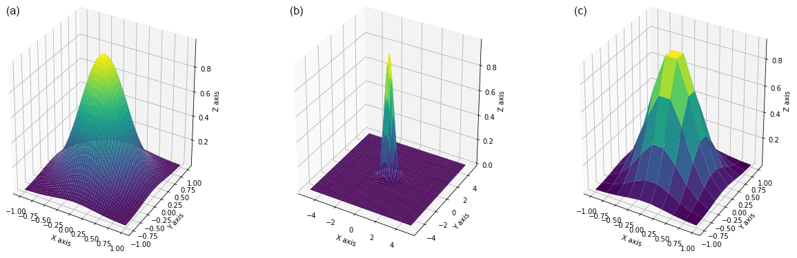
Figure A1 3D plots showing three different configurations of the Gaussian kernel with respect to the change of boundary (b) and spacing (n_x). Starting from the left: (a) $(b_{\mathrm{1}},n_{x\mathrm{1}})=(\pm \mathrm{1},\mathrm{100})$, (b) $(b_{\mathrm{2}},n_{x\mathrm{2}})=(\pm \mathrm{5},\mathrm{100})$, (c) $(b_{\mathrm{3}},n_{x\mathrm{3}})=(\pm \mathrm{1},\mathrm{10})$.