Visualization of radar-observed rainfall for hydrological risk assessment

Short-duration high-intensity rainfall constitutes a major hydro-meteorological hazard, with impacts such as pluvial (urban) flooding and debris flow. There is a great demand in society for improved information on small-scale rainfall extremes, both in real time (e.g. for early warning) and historically (e.g. for post-flood analysis). Observing this type of events is notoriously difficult, because of their extreme small-scale space-time variability. However, owing to recent advances in weather radar technology as well as integration with ground-based sensors, observational products potentially applicable in this context are now available. In this paper we present a visualization prototype tailored for hydrological risk assessment by using sub-basins as spatial units, by allowing temporal aggregation over different durations (i.e. accumulation periods) and by expressing high rainfall intensities in terms of return period exceedance. The radar-based data is evaluated by comparison with gauge observations and the quality is deemed sufficient for the intended applications. Different stakeholders have shown great interest in the prototype, which is openly accessible online.

1 Introduction

Cloudbursts, i.e. short-duration high-intensity rainfall events, are already today a major hazard, not least because of the hydrological consequences, and they are expected to become more severe in a future, warmer climate (e.g. Willems et al., 2012). An important task in climate adaptation is therefore to improve our observation systems as well as means of communicating high-resolution rainfall information. Cloudbursts are notoriously difficult to observe: gauge networks are generally not dense enough to accurately capture the peak intensities and the small-scale spatial variability; weather radar observations are uncertain with respect to intensity as well as exact space-time location (e.g. Bringi and Chandrasekar, 2001; Delrieu et al., 2009; van de Beek et al., 2016; Thorndahl et al., 2017). Much effort has been put into developing integrated products, where gauge and radar data are merged by different approaches and algorithms (e.g. Berg et al., 2016; Ochoa-Rodriguez et al., 2019). Still uncertainties remain particularly in the reproduction of high-intensity events, as shown e.g. by Schleiss et al. (2020) who found a substantial underestimation of peak intensities in radar-based estimates when compared to gauge observations.

Despite the uncertainties, we believe today's radar-based observational products can have a value for hydrological risk assessment, if presented in a suitable way. Generally, radar rainfall is presented as animations, which makes it virtually impossible to estimate temporal accumulations that are key for assessing the hydrological response. Further, even if accumulations may be obtained, their values (i.e. the rainfall depth) are difficult to relate to hydrological risk. Parzybok et al. (2011) suggested to express temporal accumulations in terms of their return period (or, equivalently, average recurrence interval, ARI) and provided examples of maps for different durations (i.e. accumulation periods) and historical events in the USA. The concept is further used in real-time in the flood forecasting system in Iowa (Krajewski et al., 2017). Lincoln and Thomason (2018) investigated the relationship between ARI values and flash floods in the eastern USA, and suggested the 2-year 3 h rainfall as a flash flood indicator.

In this paper we present a new near real-time spatio-temporal rainfall visualization tool for Sweden, which is inspired by the work cited in the previous paragraph. The tool is based on the radar-based gauge-adjusted HIPRAD product (Berg et al., 2016; van de Beek et al., 2021). The tool focuses on sub-daily durations – the user can select between 1, 3, 6 or 12 h – and it represents large accumulations in terms of their return period. A novelty as compared with existing tools, at least to our knowledge, is that spatially the rainfall is provided on hydrological sub-basin level. The tool has been co-designed together with stakeholders as well as colleagues through discussions at workshops and project meetings over the last few years. In this paper, the precision in the visualization tool is evaluated by comparison with observations from automatic stations in the Swedish meteorological network.

2 Study region and data

The study focuses on Sweden for which Olsson et al. (2019) performed a regional analysis of short-duration rainfall extremes. Based on a data set of 22-year time series (1996–2017) of 15 min rainfall from 128 automatic meteorological stations, regional depth-duration-frequency (DDF) statistics were calculated with Sweden being divided into four regions; south-western, south-eastern, central and northern. Overall, the DDF statistics are highest in south-western Sweden and lowest in northern Sweden.

The visualization tool is based on the latest version (3) of the HIPRAD product (HIgh-resolution Precipitation from gauge-adjusted weather RADar; Berg et al., 2016), described in detail and evaluated in van de Beek et al. (2021). HIPRAD3 is based on 15-min radar scans from a network of 12 C-band radars in Sweden as well as radars in neighbouring countries, converted into a 2×2 km² grid and available since 2000. The HIPRAD3 method adjusts the radar scans by first filling potential gaps from missing scans or parts of scans, advecting the instantaneous scans to 15 min accumulations using the pySTEPS algorithm (Pulkkinen et al., 2019), and applying a clutter removal filter. Finally, a gauge-adjustment algorithm is applied to reduce bias in long-term accumulations by re-scaling the radar accumulations to a reference data set (PTHBV; Johansson and Chen, 2003) within a centered 31 d moving time window. PTHBV, which includes an undercatch correction for wind losses, is defined over land and thus also the final HIPRAD3 product. In the visualization tool, HIPRAD3 is re-mapped from its grid onto the hydrological sub-basins in the national hydrological model S-HYPE (Strömqvist et al., 2012). The mapping is performed by geometric weighting of the grid cells falling within the boundaries of each sub-basin. The median sub-basin size is ∼7 km² with most sub-basins between 1 and 20 km². HIPRAD3 is produced both as a real-time product, with a latency of ∼1 h, and as a historical product. In the latter, full gauge-adjustment is performed, using the 31 d moving window described above, whereas in the former the most recent adjustment is assumed. The evaluation in this study is performed for the historical product.

In van de Beek et al. (2021), the above regional analysis by Olsson et al. (2019) was repeated, but with the time series from automatic stations replaced by the corresponding HIPRAD3 time series (period 2000–2019), taken from the grid cells covering each of the 128 stations. On the national level, for sub-hourly durations (15, 30 and 45 min; based on a moving window approach with 15 min steps) the DDF statistics based on automatic stations are underestimated by ∼10 %–30 % in the HIPRAD3 DDF statistics. For the longer durations (1, 3, 6 and 12 h), which is the focus of this study, regional differences exist but the average underestimation is 3.6 %, i.e. a distinctly better agreement than for the shorter durations. The underestimation may be partially attributed to differences in scale between stations (point value) and HIPRAD3 grid cells (4 km²).

3 Methods

3.1 Visualization tool

The visualization tool is shown in Fig. 1, using an example from 29 August 2020 when a cloudburst hit the Gotland island, located east of the southern mainland, causing flash flooding. The map of central Gotland (Fig. 1b) illustrates the sub-basin level used in the visualization. The “control panel” allows the user to select date and time as well as a duration of interest. For rainfall depths up to a return period of 2 years, the depth is represented by different green nuances, while yellow, orange and red are used to represent depths above return periods 2, 10 and 50 years, respectively (D2, D10 and D50). The depth limits associated with the different return periods can be downloaded from the tool (“Download RP Limits”; Fig. 1a). Sections “Sources” and “Overlay” are under development. When selecting a sub-basin, a diagram with hourly observations is shown with the selected period highlighted and the total depth written in the header (Fig. 1b). The observations are updated in near real-time every hour and the complete record of historical observations are available.

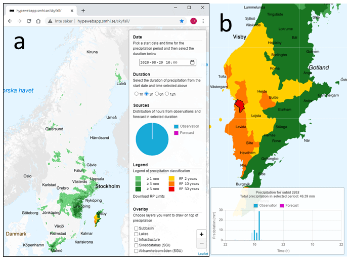
Figure 1 Rainfall over Sweden (a) and central Gotland (b) between 10:00 and 13:00 CET on 29 August 2020 as seen in the visualization tool.

3.2 Evaluation

We evaluate the performance of the HIPRAD3 visualization by comparing with the automatic stations in a multi-category contingency table approach (e.g. Wilks, 1995). The rainfall depth (D) categories are the intervals used in the visualization (Fig. 1), i.e. D<1 mm, 1 mm ≤ D < 3 mm, 3 mm ≤ D < 5 mm, 5 mm ≤ D < D2, D2 ≤ D < D10, D10 ≤ D < D50 and D≥D50 (hereafter termed D-categories). The comparison is performed for every pair of time series from station and corresponding HIPRAD3 grid cell. For each time step we identify the accompanying combination of D-categories, which becomes an entry in the contingency table; a hit requires that the D-category is the same in the automatic station and HIPRAD3, respectively. The procedure was repeated for time steps 1, 3, 6 and 12 h. Note that the regional values of D2, D10 and D50 are different for the two sources (Sect. 2); for the automatic stations the values were obtained from Olsson et al. (2019) and for HIPRAD3 the values were obtained from van de Beek et al. (2021). In the evaluation we use data from the whole available period (2000–2019) but only for the summer half year (May–October), to minimize any occurrence of solid precipitation.

A known limitation of radar-observed rainfall is that the timing may be shifted as compared with ground observations, i.e. high intensities may be recorded some time before or after it was registered on the ground. To investigate this effect, we repeated the above multi-category contingency table analysis, but this time allowing a temporal error margin of 1–3 h in HIPRAD3. Thus, if the D-category in the automatic station agrees with the HIPRAD3 D-category within the temporal error margin, it is registered as a hit in the contingency table.

4 Results and discussion

The results of the evaluation are summarized in Tables 1 and 2. As the results do not show any clear regional dependence the tabulated values are averages over all four regions from Olsson et al. (2019), i.e. entire Sweden. Looking first at Table 1, the values in columns “same cat.” represent the hit rate, i.e. the fraction of all “HIPRAD3 D-category time steps” (i.e. time steps when the HIPRAD3 depth belongs to the category in the left column) that agrees with the D-category in the corresponding automatic station. For example, out of all the 1 h time steps when the HIPRAD3 depth was in category “5 mm ≤ D < D2”, in 32.5 % of these time steps also the depth in the automatic station was in category “5 mm ≤ D < D2”, i.e. hits. For the different durations, the hit rate generally ranges from 40 %–50 % for category “1 mm ≤ D < 3 mm” to 10 %–20 % in category “D10 ≤ D < D50”. For category “5 mm ≤ D < D2”, the hit rate increases with duration, which reflects that the interval of this category increases as D2 becomes gradually larger for longer durations.

Table 1 Fraction (%) of time steps where the D-category of the automatic station either agrees with the one of HIPRAD3 (column “same cat.”, equivalent to hit rate) or is within ± one D-category (column “± one cat.”), for durations 1, 3, 6 and 12 h.

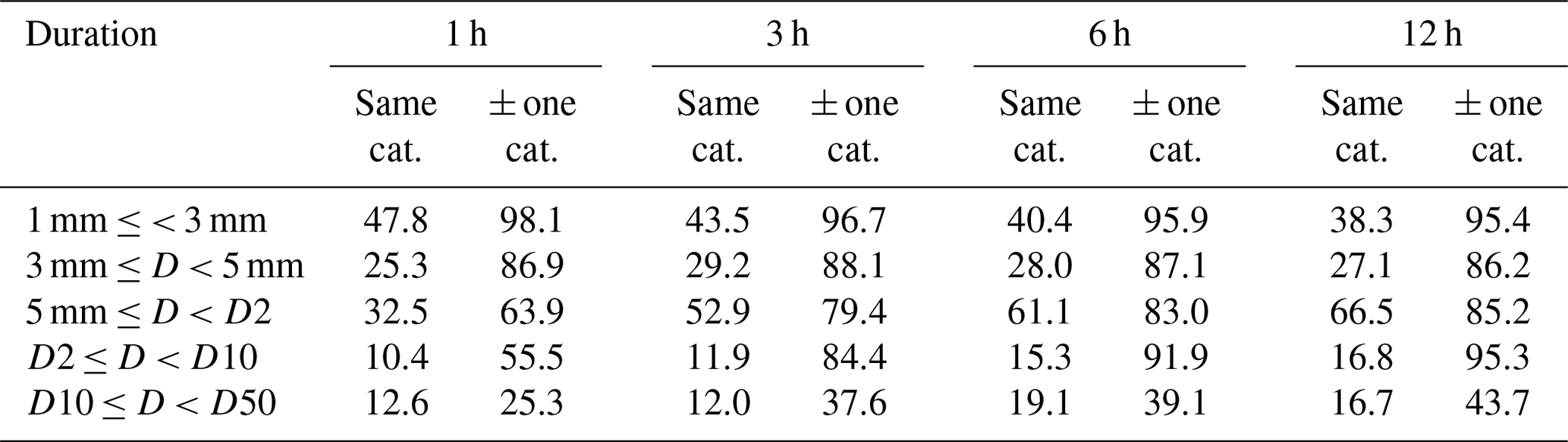
Table 2 Fraction (%) of time steps where the D-category of the automatic station agrees with the one of HIPRAD3 when allowing an error margin of 1, 2 and 3 h, for durations 1, 3, 6 and 12 h.

For the lower D-categories, in ∼50 % of the time steps the station observation is below the HIPRAD3 interval and in ∼15 % it is above. For the higher D-categories, the corresponding numbers are ∼80 % and ∼5 %. HIPRAD3 thus generally overestimates the depth, compared with the stations, and this result may seem to be in conflict with other studies concluding that radar-based observations generally underestimate rainfall depths, especially high or extreme depths (e.g. Schleiss et al., 2020). When evaluating radar-based observations, normally station observations are taken as the reference and compared with what the radar observes at the same time and place. In this perspective the radar-based observations will generally underestimate the station observations, e.g. because of space-time uncertainty/errors. Here we do the analysis in the opposite way; we use HIPRAD3 as the reference and compare with what the station observes at the same time and place. Because of space-time uncertainty, in this perspective the radar-based observations will instead generally overestimate the station observations, as (high) rainfall is displaced (in time and/or space) and the corresponding station observation will generally be lower.

The values in column “± one cat.” in Table 1 represent the fraction of time steps when the D-category in the automatic station is within ± one category, as compared with the D-category in HIPRAD3. For example, out of all the 1 h time steps when the HIPRAD3 depth was in category “5 mm ≤ D < D2”, in 63.9 % of these time steps the depth in the automatic station was in either category “3 mm ≤ D < 5 mm”, category “5 mm ≤ D < D2” or category “D2 ≤ D < D10”. The values in column “± one cat.” generally increase with increasing duration, and further the rate increases with increasing D-category. For durations 6 and 12 h, the D-category in the automatic station is very often within ± one category of HIPRAD3, except for “D10 ≤ D < D50” where the percentage is ∼40 %.

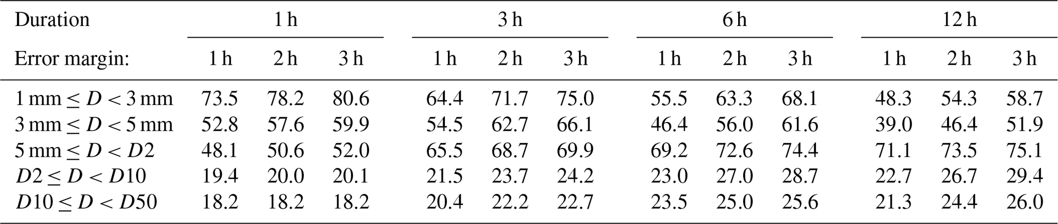
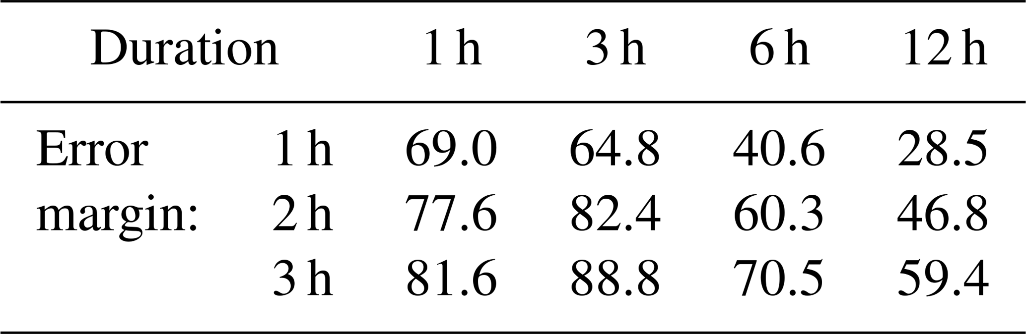
The impact of allowing a temporal error margin is shown in Table 2, where the fractions correspond to the ones in columns “same cat.” in Table 1, but calculated using error margins 1, 2 and 3 h. For example, out of all the 1 h time steps when the HIPRAD3 depth was in category “5 mm ≤ D < D2”, in 48.1 % of these time steps also the 1 h depth in the automatic station was in category “5 mm ≤ D < D2” if allowing a 1 h error margin (i.e. if looking at a 3 h time window centred on the time step under investigation). As expected, the fractions increase with increasing error margin. For single combinations of D-category, duration and error margin, the relative increase ranges widely from 7 % (D-category “5 mm ≤ D < D2”, duration 12 h, error margin 1 h) up to 137 % (“3 mm ≤ D < 5 mm”, 1, 3 h). As the relative increase has no clear dependence on D-category, in Table 3 the increase is averaged over all D-categories to more clearly show the overall impact of the error margin. The relative increase is similar for durations 1 and 3 h, and then gradually decreases for 6 and 12 h. This reflects the fact that the impact on the accumulated depth of shifting a time window a few steps back or forth in time is higher the shorter the time window.

Table 3 Relative increase (%) of the hit rate (values in columns “same cat.” in Table 1) when allowing a temporal error margin between 1 and 3 h.

The results in Tables 1–3 indicate the precision with which HIPRAD3 is able to describe local rainfall, as represented by the automatic stations. The ability of HIPRAD3 to identify the correct category at a given time step is limited, as shown in Table 1, but if allowing an error margin in terms of depth and/or time the performance increases substantially. This suggests that a more qualitative presentation may be more sensible, where depths are grouped into fewer categories and time intervals are given rather than exact time steps. On the other hand, in many situations it can be expected that users can “validate” the HIPRAD3 estimates, e.g. by using municipal or private observations, and that way assess the accuracy for a specific event. For this reason, it may be unfortunate to “degrade” the information content provided in the visualization tool.

There are some aspects that most likely have had some impact on the evaluation. One is that HIPRAD3 includes an undercatch correction that is not applied to the automatic stations. For this reason, HIPRAD3 should show systematically somewhat higher values particularly at small depths (i.e. low D-categories) and long durations, where the effect of undercatch is most prominent, especially in the north where precipitation falls as snow also in parts of the summer half year considered here. Another aspect is differences in spatial scale. Firstly, we compare 2×2 km² gridded observations (HIPRAD3) with point observations (stations). This mismatch adds uncertainty especially at large depths and short durations, associated with small-scale events where the areal reduction effect may be notable (e.g. Svensson and Jones, 2010; Eggert et al., 2015; Thorndahl et al., 2019). Secondly, the evaluation is performed on HIPRAD3 grid scale (4 km²) whereas the visualization is performed on S-HYPE sub-basin scale (median size ∼7 km²; Sect. 2). For sub-basins substantially larger than the median value the results from this evaluation may not be fully representative. We neglect these aspects in this study, but we intend to perform more detailed evaluation in the future.

5 Concluding remarks

We present a rainfall visualization tool focused on providing support for hydrological risk assessment, particularly associated with sub-daily high-intensity rainfall events. The tool uses a sub-basin spatial resolution, allows for analysis of different temporal accumulations and presents large rainfall depths in terms of return periods. The uncertainties involved as well as the effects of allowing error margins in terms of depth and time were quantified in an evaluation.

Despite the uncertainties involved, we believe the tool has an obvious value for hydrological risk assessment, depending on the purpose and conditions. This has been confirmed in communication with various stakeholders, e.g. in joint evaluations of well-known extreme events with societal consequences (e.g. in Jönköping 2013, Malmö 2014 and Hallsberg 2015). If observed rainfall events can be “validated” against independent ground observations (or impacts), the visualization is conceivably useful for post-analyzing e.g. flood events. If no independent observations are available, the visualization of an event should be considered a “best guess” where the exact depths as well as the space-time evolution must be viewed with caution, especially for high-intensity events. Furthermore, current testing indicates that HIPRAD3 can be successfully used to force 1 h simulations with the national hydrological S-HYPE model, which supports its applicability for hydrological assessment. However, HIPRAD is under constant development and will gradually improve by e.g. better conversion from reflectivity to intensity, more effective estimation of missing data and incorporation of observations from additional sensors (van de Beek et al., 2021).

Finally, we intend to develop the tool in different ways. One is to include visualization of other sensors, such as gauges, X-band radar and microwave links, as well as blended products, potentially at higher space-time resolutions. Another is to combine the observations with high-resolution rainfall forecasts into a seamless stream. Conceivably a nowcasting approach is preferable, to allow a smooth transition from the observations, and different options are currently being developed and evaluated. A third way is to include relevant GIS layers in the tool, e.g. maps representing risk of landslide or other hazards related to intense rainfall.