Development of an empirical model for seasonal forecasting over the Mediterranean

In the frame of MEDSCOPE project, which mainly aims at improving predictability on seasonal timescales over the Mediterranean area, a seasonal forecast empirical model making use of new predictors based on a collection of targeted sensitivity experiments is being developed. Here, a first version of the model is presented. This version is based on multiple linear regression, using global climate indices (mainly global teleconnection patterns and indices based on sea surface temperatures, as well as sea-ice and snow cover) as predictors. The model is implemented in a way that allows easy modifications to include new information from other predictors that will come as result of the ongoing sensitivity experiments within the project.

Given the big extension of the region under study, its high complexity (both in terms of orography and land-sea distribution) and its location, different sub regions are affected by different drivers at different times. The empirical model makes use of different sets of predictors for every season and every sub region. Starting from a collection of 25 global climate indices, a few predictors are selected for every season and every sub region, checking linear correlation between predictands (temperature and precipitation) and global indices up to one year in advance and using moving averages from two to six months. Special attention has also been payed to the selection of predictors in order to guaranty smooth transitions between neighbor sub regions and consecutive seasons. The model runs a three-month forecast every month with a one-month lead time.

1 Introduction

Dynamical models for seasonal forecasting have noticeably improved during the last decades mainly due to the advance, both in the estimate of the atmospheric initial conditions as well as the model physics supported further by computing capabilities. However, they still show low skill over extratropical latitudes (Kim et al., 2012). The surroundings of the Mediterranean Sea are specially affected by this low skill, due either be to lack of predictability or to errors in forecasting systems, being exacerbated by its complex orography and land-ocean distribution (Weisheimer et al., 2011; Doblas-Reyes et al., 2013). Besides, the Mediterranean region is located in a transition zone between the arid belt of Northern Africa and the temperate zones over Europe. Another distinctive feature is the type of precipitation: over most of the domain, a high fraction of annual precipitation is convective, implying high spatial and temporal variability. The average expected precipitation for a three months period can be reached in one single day for particularly intense events (Toreti et al., 2010). In this context, the Mediterranean Services Chain based On Climate PrEdictions (MEDSCOPE) project (see https://www.medscope-project.eu, last access: 19 August 2019) and others, developed under initiatives like the European Research Area for Climate Services (ERA4CS) (see http://www.jpi-climate.eu/ERA4CS, last access: 19 August 2019) aim at improving Climate Services over this region, searching for new sources of predictability and developing different tools and products. In particular, one of the MEDSCOPE work packages consists of a collection of sensitivity experiments designed to explore new sources of predictability that may lead to improvements in our understanding of mechanisms and processes involved at seasonal timescales. As result of the sensitivity experiments conducted within the MEDSCOPE project, new specific predictors will be proposed for the Mediterranean region. A by-product of this exploration will be the development of an empirical seasonal forecasting system bringing together predictors coming from new sources of predictability unveiled by the sensitivity experiments.

Choosing the model

Here we present a preliminary (beta) version of the empirical seasonal forecasting system. The purpose of this beta version is twofold: first, establish a reference version based on standard predictors making use of known sources of predictability and, second, compare its skill over the Mediterranean with the state-of-the-art dynamical systems. Results coming from ongoing work within the project providing new specific predictors for the Mediterranean region can be easily added to this preliminary version. The skill of the new system will be evaluated with respect to this reference version. Eden et al. (2015) developed a global empirical seasonal forecasting system based on Multi Linear Regression (MLR), using a few global climate indices as predictors, and producing a probabilistic output using the residuals from regression. This system shows ability to produce skilful forecasts over several world regions, despite the reduced number of predictors used. Wang et al. (2017) showed, using MLR too, that a careful selection of predictors can produce skilful prediction of winter NAO.

The beta version of the empirical seasonal forecasting system here described follows the same procedure based on MLR suggested by these two studies as this kind of models only requires very modest computing resources and has the additional advantage of being easy to modify. The second version of the empirical seasonal forecasting system, incorporating results from MEDSCOPE project findings, will be developed and evaluated in the second part of the project.

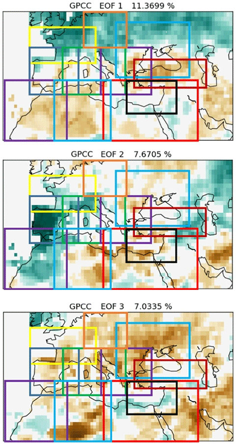
Figure 1 Domains for predictor's selection proposed in this study. First three Empirical Orthogonal Functions (EOFs) of annual precipitation (GPCCv7 data) over Mediterranean domain are represented as background.

2 Methodology

2.1 Division in sub regions

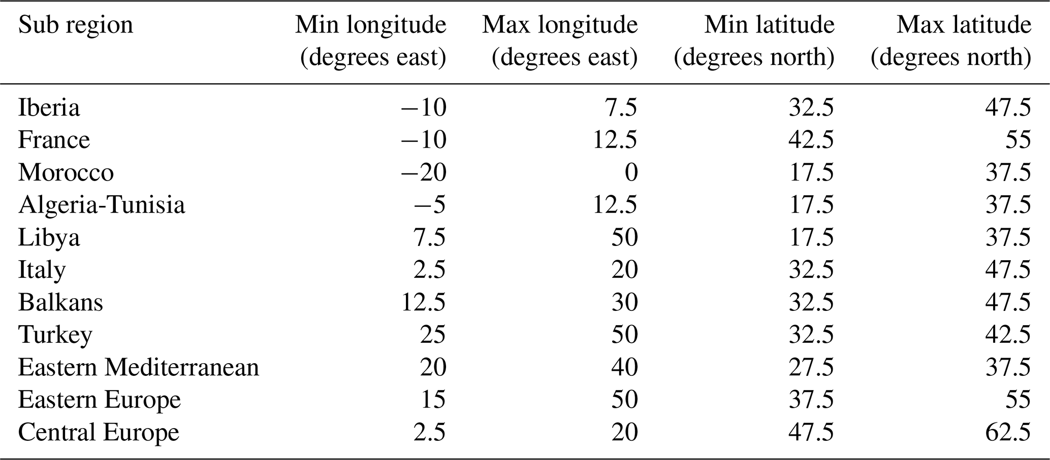
Given the extension of the Mediterranean domain, its great complexity (both orographic and land-ocean distribution), and location, sub regions within the domain are affected by different factors at different times of the year. In order to improve the skill of the system, the empirical model will use different sets of predictors for every climatologically homogeneous defined sub region within the Mediterranean domain and every season. Selection of predictors, from the pool listed in Table 1, is based on their high correlation with precipitation over large areas within the sub region and for each particular season. One issue with this type of models where predictors may change spatially is the extreme noisiness of the forecasts showing very different results for neighbour grid points. For example, probability values for lower tercile over a grid point in southwestern Turkey are calculated for 2018 FMA using 2 different sets of predictors (Table S1 in the Supplement, row FMA, columns Turkey and East Mediterranean), obtaining 61 % and 37 %. As a compromise between selecting the best predictors for every point and forecasting smooth synoptic scale anomaly patterns, the domain is divided in sub regions (see Table 3), and a subset of predictors from the pool (see Table 1) will be selected for each one of them as a whole. To avoid abrupt transitions in space and time, predictors will be restricted to partially match among neighbour sub regions and consecutive seasons (for example, January–March and February–April). To further smooth out transitions among sub regions, they have been defined with a high amount of overlap. Those grid points belonging to more than one sub region will be assigned a weighted average from values from different sub regions, based on distance to respective borders.

Table 1 List of the initial pool of predictors (25) (and their incremental values) based on atmospheric (A), oceanic (O) climate variability indices and snow cover (S). Definition and data are available at the indicated webs.

^∗ Calculated from https://climexp.knmi.nl/NCDCData/ersstv4.nc (last access: 19 August 2019) as defined at https://stateoftheocean.osmc.noaa.gov/sur/atl/tasi.php
(last access: 19 August 2019).

In short, sub regions have been defined seeking a compromise between encompassing main land areas and countries (adding an overlap area among them) and climatological homogeneity. In order to meet this last feature, empirical orthogonal functions (EOFs) for yearly precipitation have been calculated and their patterns taken into account for defining sub regions. Figure 1 depicts these three EOFs with chosen sub regions superimposed. Table S1 provides the exact definition of 5 sub-regions employed.

Table 2 Percentage of grid points showing significant correlation [for p-value ≤ 0.10] between Dipole Mode Index (DMI) (and its incremental values) and January–March and February–April precipitation (GPCCv7). Table explores different moving averages (up to 6 months) and lead-months for predictors (up to 10 months). Bold numbers correspond to percentages higher than 30 %, and italic higher than 20 %.

2.2 Choosing predictands

As we intend to deliver synoptic scale anomaly patterns, low-resolution predictands will be selected for this beta version of the system. Precipitation data from the Global Prediction Climate Centre (GPCC) dataset (Schneider et al., 2017) will be used (2.5^∘ version). Data consist of a blend of GPCC v7 (until 2013) and its monitoring (v5) from 2014 onwards. Surface temperature is obtained from the ERA-interim reanalysis (Dee et al., 2011). The period selected is 1979–2016. In both cases, predictands will consist of the three months average for every season and grid point. The empirical model runs every month with one-month lead time, i.e., computing a forecast for the following season (3 months) and for both predictands. For example, in January, the forecast will be calculated for February–March–April.

2.3 Exploration of predictors

This beta version of the empirical model makes use of global climate indices provided by external sources. The initial pool of predictors includes 25 monthly time series of indices associated to atmospheric and oceanic climate variability indices, ocean heat content and snow cover (see Table 1). Additionally, for each index, a new monthly time series is generated calculating the incremental value from the previous month (e.g., February incremental value would be February minus January). The purpose of such incremental series is try to find additional sources of predictability by analysing if a rapid change in the state of a certain indicator could be linked to anomalous atmospheric circulation. Before exploring these 50 indices (25 climate indices plus their 25 incremental series), moving averages from 2 to 6 months are applied, to better capture mechanisms from different time scales.

The selection process of predictors for each sub region starts by the computation for each season of the correlation coefficient between predictand and predictors from the pool applying different lead times (from 1 to 12 months). Correlation is also computed for six different options of moving average (up to 6 months). So, for a particular grid point, predictor and season, a collection of correlation coefficient values will be obtained. A predictor is finally selected considering the percentage of grid points with significant (for p-value ≤ 0.10) correlation. As an example, Table 2 shows percentage of points with significant correlation for the predictor DMI for different lead times and moving averages.

Bearing in mind the known relative low predictability, and consequently skill, for the studied area, this procedure will try to unveil the best possible signal that a predictor from the pool can offer playing with different lead times and moving averages. Considering correlation data from the different predictors in Table 1, and applying constrains for the sake of continuity among regions, a set of predictors is finally selected for every region (see Table S1).

2.4 Running the model

The model makes use of multiple linear regression (MLR), as described in Wilks (2006), over every grid point, using the set of predictors selected for each specific sub region. Trend is removed before calculating regression and then added to regression results. In order to express the forecast in probabilistic terms, first, terciles are calculated for predictands at every grid point. Then, probabilities are assigned to every tercile, using a normal distribution, centred in the deterministic output of the MLR and using information from residuals to adjust its width. This distribution represents the expected probability density function (pdf) for the forecasted predictand value. The computation of the area below this curve and between observed terciles provides the probability of the forecasted value to be in every one of them (Eden et al., 2015).

This procedure requires predictands to adjust to a normal distribution. As this is not the case with precipitation, square root is previously applied over this predictand, to transform it into a normal-like distribution (Pasqui et al., 2007). Additionally, the system performs a series of checks to ensure that certain required assumptions are met, such as: no collinearity among predictors, no overfitting, residuals are normally distributed and homoscedastic and do not show autocorrelation.

2.5 Verification of results

The performance of the empirical model is assessed by verifying against observational grids for a hindcast calculated for the period 1983–2014. Additionally, the verification scores computed for the empirical system are compared with those of some state-of-art seasonal forecasting systems based on dynamical models for a common hindcast period to check the possible benefit of the empirical method here described. Regression is trained for same period, using “Leave-One-Out” technique (Wilks, 2006), excluding a total of 5 years from the series (two before and two after the year we are forecasting) to avoid possible autocorrelation (Breusch, 1978 and Godfrey, 1978). Section 3.3 describes several verification indices calculated for this version of the empirical system, and their comparison with the corresponding indices calculated from dynamical models.

3 Results

3.1 Precipitation and temperature forecasts

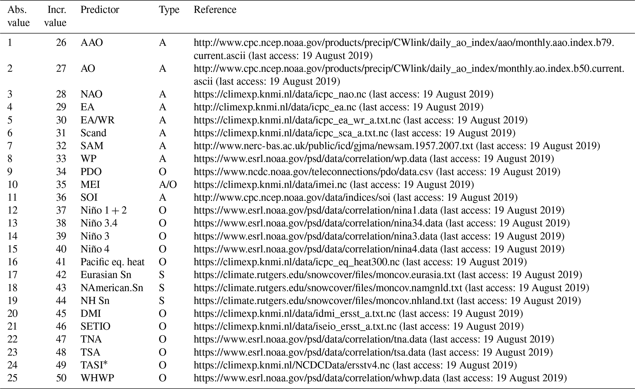
Figure 2 shows a few examples of forecasts maps for precipitation. Although some noisy features can still be seen over certain areas, mainly Egypt and Arabian Peninsula, observed patterns are synoptic scale and continuous, generally speaking. Borders between sub regions are not evident, either, so forecast maps are reasonably shaped, and defined sub regions and proposed constraints for predictors seem to work well (all this set up were imposed to produce smooth synoptic scale anomaly patterns) This particular example corresponds for the 1-month lead time 2014 DJF and JAS forecast, and anomaly patterns resemble in terms of structures and spatial variability those shown by dynamical models. In order to compare results, the empirical model is also run using temperature as predictand and using the same predictors as for precipitation, under the assumption that same anomalous circulation captured by these predictors can affect to temperature as well. Results can be seen in Fig. 3. The same conclusions about the forecasts appearance also applies for temperature.

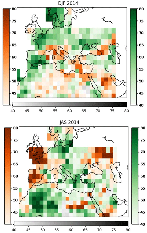
Figure 2 Example of precipitation forecasts. Probability for the most likely tercile is shown at every grid point. Green (orange) corresponds to upper (lower) tercile.

Figure 3 Example of temperature forecasts. Probability for the most likely tercile is shown at every grid point. Red (blue) corresponds to upper (lower) tercile.

3.2 Verification

Verification scores are computed and visualized following (Sánchez-García et al., 2018). For every predictand (temperature and precipitation), season, score and verifying sub region, results from a selection of seasonal forecasting systems based on dynamical models and the empirical system are put together in a table for easy comparison.

The dynamical models and versions used for this comparison were operational when this project started (2017) and are the following: ECMWF system 4, Météo-France system 5, Met-Office system 9 (GloSea5), National Center for Enviromental Prediction (NCEP) system version 2, Canadian Seasonal to Inter-annual Prediction System (CanSIPS) and Japanese Seasonal Forecasting System 2. Both probabilistic and deterministic scores have been computed for dynamical models and the empirical system: Ranked Probability Skill Score (RPSS), Relative Operating Characteristic (ROC) area and Brier Skill Score (BSS), for upper and lower tercile probabilities and anomaly correlation. Statistical significance of all computed scores has been quantified by the p-value estimated using a bootstrapping non-parametric method (see details in Wilks, 2006).

Table 3 Sub regions used in the seasonal forecasting empirical system.

To compare the skill of this first version of the empirical model against this selection of dynamical models is necessary to choose a common period of hindcast data, to ensure that differences in scores are not attributable to changes in predictability over the years. So, although hindcast for the empirical system is available for a longer period, skill is evaluated for the common period 1997–2009. Table 4 shows some examples for the scores anomaly correlation, RPSS and ROC area (lower and upper tercile) computed for precipitation over France and for temperature over the Eastern Mediterranean region. For these particular areas, the empirical system performs especially well. Generally speaking, precipitation scores for the empirical system are better than for dynamical models. Temperature scores are roughly the same level for dynamical models and empirical system. Additionally to tables for specific sub regions, Fig. 4 depicts some examples of anomaly correlation maps for precipitation calculated for 1983–2014 and for autumn (SON) and spring (MAM) seasons. Certain areas like northern France, Benelux, parts of Germany or Morocco, large areas of Eastern Mediterranean and west of Black Sea show good correlation with observations for these particular two examples. However, other places, e.g., most of Iberian Peninsula and Italy, most of the Eastern part of the domain for SON and large parts of Northern Africa for MAM, hardly show any. The relatively high skill reached over some regions show the potential of the empirical system. As there is still room for improvement, additional efforts should focus on the identification of good predictors for large areas still showing low skill.

Table 4 (a) Selection of verification scores (anomaly correlation coefficient (upper left), Ranked Probability Skill Score (RPSS) (upper right), and Relative Operating Characteristic area (ROC Area) for lower/upper tercile (bottom left/right) for seasonal forecasted precipitation over France (41–52^∘ N, 6.4^∘ W–10^∘ E). Every table contains information of an individual verification score, representing each cell the average value of the corresponding score over the selected verification domain (France) for a particular model (y-axis) and 1-month lead time forecasted season (x-axis). The uppermost row in all tables corresponds to the empirical seasonal forecasting system. GPCC precipitation data are used as verifying observations. Statistical significance of all computed scores has been quantified by the p-value [(^∗) for p-value ≤ 0.05; (#) for 0.05 < p-value ≤ 0.1] estimated using a bootstrapping non-parametric method (Wilks, 2006). (b) Same as Table 3 but for temperature, East Mediterranean (20–40^∘ N, 27.5–62.5^∘ E) domain and ERA-Interim temperature for verifying observations.

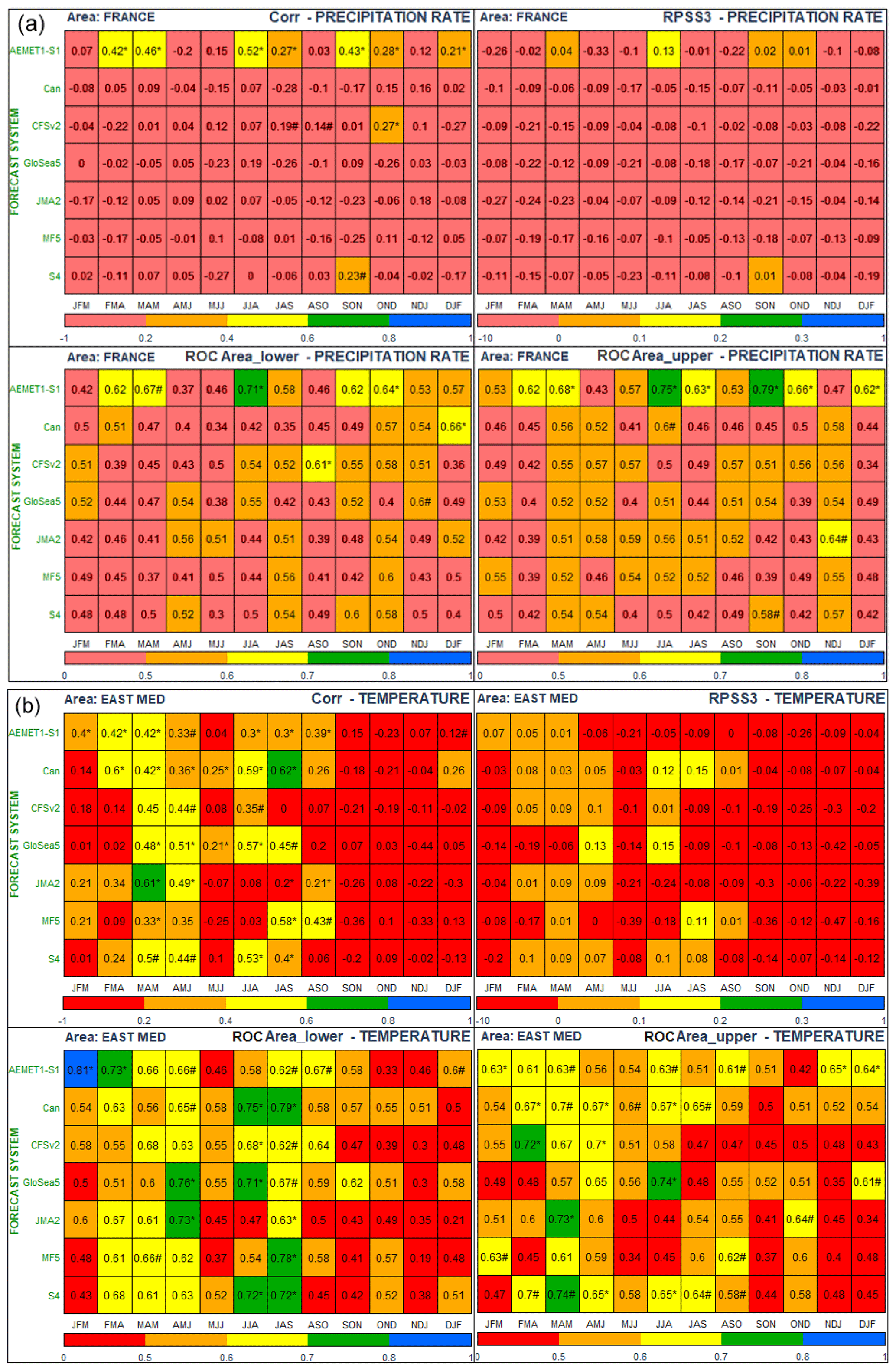
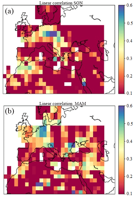
Figure 4 Anomaly correlation between empirical model forecasts and observed precipitation (GPCCv7) for autumn (SON) (a) and spring (MAM). The hindcast period covers 1983–2014.

4 Conclusions

Major research and climate services initiatives support advances in seasonal forecasting. In the frame of MEDSCOPE project, we present here a beta version of a seasonal forecast empirical system intended as reference version using as predictors mainly well-known climate variability indices. Next version will add new predictors based on a collection of targeted sensitivity experiments – conducted also in the frame of the MEDSCOPE Project – for exploring predictability over the Mediterranean region. The proposed system is valuable as a starting point, and the addition of new predictors resulting from targeted experiments will be rather straightforward. Bearing this in mind, the code has been designed in such a way to facilitate both either modification or incorporation of new predictors.

As indicated earlier, the nature and appearance of spatial patterns observed on the forecasts seems to fulfil the original aim of producing both synoptic scale structures and continuity among regions. Furthermore, as we have discussed, this beta version has also some merit in itself – not only as a reference version to check the improvements of further developments – as it performs better than state-of-the-art seasonal forecasting systems based on dynamical models for certain seasons and over certain regions. Nevertheless, with regard to other regions, skill is still poor and comparable or below dynamical models. Plausible causes for this result may be attributed to the fact that selection of predictors was made subjectively and only for precipitation. Besides, selection was based in linear correlation between predictors and accumulated precipitation, whereas the model uses its square root. Another possible cause explaining low performance is related with the procedure for selection of predictors, as it checks the percentage of points showing some signal within a region, but does not take into account where that signal is: it may be possible that all predictors show signal over the same part of the region, and at the same time, it may not exist any good predictor for other parts. Next version of the system will implement an automatic procedure for selection of predictors, and efforts will focus on developing an objective procedure that cover the issues above described.

On the other hand, the fact that selected predictors for temperature are the same than for precipitation is a serious limitation of the empirical model. We expect better results when making an independent selection of proper predictors for this predictand. Nevertheless, present results are encouraging, with scores being roughly at the same level as for dynamical models. In any case, using the same predictors for temperature and precipitation makes easier to analyse circulation anomalies for the incoming season and its physical interpretation.

Therefore, this first version of the model shows relatively good results and at least of similar skill as dynamical models. Improvements currently being developed and planned for the empirical system and the expected new specific predictors from MEDSCOPE will be implemented in the next version of the system. The new version is expected to be an additional and reliable source of information to be used in combination with dynamical models and aiming at improving the skill of seasonal forecasts over the Mediterranean region.