 | 13 Jul 2021
Climate change projections of maximum temperature in the pre-monsoon season in Bangladesh using statistical downscaling of global climate models
M. Bazlur Rashid
Syed Shahadat Hossain
M. Abdul Mannan
Kajsa M. Parding
Hans Olav Hygen
Rasmus E. Benestad
Abdelkader Mezghani
The climate of Bangladesh is very likely to be influenced by global climate change. To quantify the influence on the climate of Bangladesh, Global Climate Models were downscaled statistically to produce future climate projections of maximum temperature during the pre-monsoon season (March–May) for the 21st century for Bangladesh. The future climate projections are generated based on three emission scenarios (RCP2.6, RCP4.5 and RCP8.5) provided by the fifth Coupled Model Intercomparison Project. The downscaling process is undertaken by relating the large-scale seasonal mean temperature, taken from the ERA5 reanalysis data set, to the leading principal components of the observed maximum temperature at stations under Bangladesh Meteorological Department in Bangladesh, and applying the relationship to the GCM ensemble. The in-situ temperature data has only recently been digitised, and this is the first time they have been used in statistical downscaling of local climate projections for Bangladesh. This analysis also provides an evaluation of the local data, and the local temperatures in Bangladesh show a close match with the ERA5 reanalysis. Compared to the reference period of 1981–2010, the projected maximum pre-monsoon temperature in Bangladesh indicate an increase by ∘C in the near future (2021–2050) and ∘C in the far future (2071–2100) assuming the RCP8.5/RCP4.5/RCP2.6 scenario, respectively.
- Article
(4206 KB) - Full-text XML
-
Supplement
(250 KB) - BibTeX
- EndNote


1.1 Background
Bangladesh is highly vulnerable to climate change due to its flat and low-lying delta landscape, dependence upon agriculture, high population density and poverty. Natural disasters and extreme weather events, such as floods and heat waves, occur frequently and are often detrimental to lives and livelihoods. Reliable information about how regional and local climates have changed in the past and may change in the future is important for managing climate change risks.
Global climate models (GCMs) can provide future projections of climate variables (Stocker et al., 2013) but typically at a coarse resolution that is of limited use in impact studies assessing the local response to global climate change. These projections can nevertheless provide some important information about large-scale climate change. A common way of approaching the question of local climate change is through so-called downscaling where information about large-scale climate change is combined with information about how the local climate depends on the large-scale situation and local geographical factors (Benestad, 2016). One implicit assumption of downscaling is that the climate models have a minimum skillful scale that is different from the spatial resolution (Takayabu and Hibino, 2016), and that the local details have a predictable dependency on the large-scale features that the model is able to reproduce. Some explanations for the models' minimum skillful scales include their simplicity and idealistic representation of the world, their use of discrete numbers and imperfect numerical algorithms for solving mathematical operations, a lack of small-scale surface details, the presence of unresolved small-scale processes, and an imperfect model design due to our limited understanding of the climate system. There are two main approaches to downscaling GCM results to higher spatial resolutions: dynamical downscaling using regional climate models (RCM) (Rummukainen, 2010) and empirical-statistical downscaling (ESD) in which a statistical connection is established between the large-scale climate and local response (Hewitson et al., 2014). Dynamical downscaling is based on physical-dynamical relationships and provides a comprehensive picture of the climate, which makes it well suited for climate process studies (Giorgi and Gutowski, 2015; Kjellström et al., 2007). One main disadvantage with RCMs is the high computational demand which tends to limit the downscaling to one or a small set of GCM simulations (Gutman et al., 2012), but there are also other caveats such as mismatch between the driving GCM and the RCM (von Storch et al., 2000) and the need for bias-adjustment (Gudmundsson et al., 2012; Maraun, 2013). ESD on the other hand is computationally cheap and can easily be applied to a large GCM ensemble, but requires long observational time series and typically downscales each climate variable separately (Maraun and Widmann, 2018; Benestad et al., 2009). The assumption of a stationary statistical relationship is essential to obtain trustworthy projections for future periods in ESD, but this assumption is also implicitly made for GCMs and RCMs which rely on statistical parameterization schemes to represent some of the many complex physical processes that govern the climate.
Various methods can be used in ESD, such as analogue methods and circulation typing, regression analysis, or neural network methods (Wilby et al., 2002; Maraun et al., 2015). The statistical model is typically calibrated on historical observations and then applied to GCM results to generate output for future climate scenarios to study the impact of climate change on a regional scale (Wilby et al., 2004). There are two different approaches in ESD: (1) training the statistical model on each time step (e.g., daily weather charts and daily temperature) to downscale the local “weather”; (2) aggregating statistical aspects such as the mean μ and standard deviation σ over a season to downscale the parameters of probability density functions describing the local “climate” (Benestad, 2016). Bias adjustments such as quantile mapping are often used to correct for systematic biases in global or regional climate model simulations, and can be seen as a simple and non-parametric statistical downscaling method (Gudmundsson et al., 2012; Gutjahr and Heinemann, 2013) which attempts to adjust the distribution of historical model data such that it matches the distribution of the observations, hence, it does not require a prior knowledge of the theoretical distribution of the weather variables. Large-scale features can be represented in different ways in ESD, either based on the nearest grid-box values from reanalyses and GCMs (e.g., Liu et al., 2016), or by an index that represents some spatially aggregated quantity or a statistic describing the spatio-temporal patterns in a larger region (e.g., Benestad, 2011). Common Empirical Orthogonal Function (common EOF) analysis applied to GCM and reanalysis data can be used to represent the large-scale predictors (Flury, 1988; Barnett, 1999; Benestad, 2001, 2011). This means that EOF analysis is applied to an object combining the GCM and reanalysis data, which decomposes the combined data into a common set of spatial patterns, eigenvalues representing the relative importance of each pattern, and principal components (PCs) describing the temporal variations associated with the spatial patterns for the GCM and reanalysis data separately (see schematic in Fig. 1). In ESD, the part of the PCs that represents the reanalysis is used to tune the statistical downscaling model which is subsequently applied to the part of the PCs that represents the GCM data to obtain future projections. The method ensures that the exact same large-scale spatial structures are identified in both data sets. The common EOFs can also facilitate an evaluation of the GCMs' ability to reproduce the spatio-temporal covariance structure found in the reanalysis through a comparison between the part of the PCs that represents the reanalysis and GCM, respectively (Benestad et al., 2016). Usually, one set of common EOFs is estimated for each combination of reanalysis and GCM simulation.
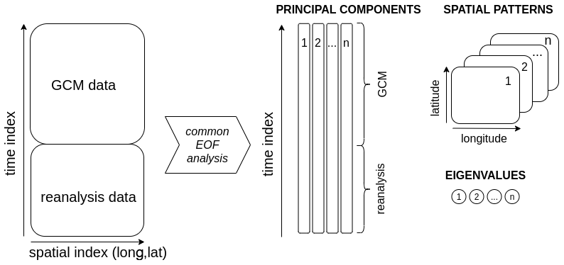
Figure 1Schematic representation of the common Empirical Orthogonal Function (common EOF) analysis. The figure shows how EOF analysis is applied to a mixed object containing GCM and reanalysis data joined along the time axis, deconstructing the data into a set of n spatial patterns, eigenvalues representing the relative strength of the patterns, and principal components representing the temporal variations associated with the patterns.
Bangladesh has been the subject of some statistical downscaling studies. Rahaman et al. (2015) found that a statistical downscaling model (SDSM) showed good agreement between observed and simulated maximum and minimum temperatures, indicating that the method can be used to predict future scenarios with some confidence. For precipitation, on the other hand, their results were not in such a good agreement. Nury and Alam (2013) downscaled temperature and precipitation for Northeastern Bangladesh from the HADCM3 model, using a similar method and found reasonable agreement between observed and downscaled data. Shourav et al. (2016) used SDSM to downscale future climate projections over the city of Dhaka, Bangladesh. Their study indicated that climate change will cause continuous increases in rainfall, temperature, and related extreme events. Pour et al. (2018), using a Support Vector Machine (SVM) based Model Output Statistics (MOS) approach (i.e., relating GCM model outputs to observational data, see Glahn and Lowry, 1972 or Maraun and Widmann, 2018), downscaled 4-GCM simulations that were selected to cover the whole range of projections. Considering four different emission scenarios, they reported an increase in annual mean precipitation in almost all parts of Bangladesh for all scenarios, but a stronger increase in the western part of Bangladesh. Alamgir et al. (2019) also used an SVM method to establish downscaling models of minimum and maximum temperature in Bangladesh which were based on 8 GCM simulations. The downscaled projections showed a significant increase in temperature during the 21st century, with the minimum temperature increasing in winter (December–February) and the maximum temperature increasing in the pre-monsoon summer season (March–May). Khan et al. (2020) studying an ensemble of 11 RCM simulations projected a shift in the spatial patterns of drought in the pre-monsoon period in the coming century. All these past studies have involved a small number of GCM simulations, which can be problematic because small ensembles do not give a representative picture due to the presence of random noise (Mezghani et al., 2019).
There are examples of studies using GCMs or RCMs to evaluate the local response to global climate change in Bangladesh, but in general the spatial resolution has been too coarse for many impact studies. Using 11 GCMs, OECD (2003) estimated that by 2100, the average temperature in Bangladesh would increase by 2.4 ∘C following the SRES B1 scenario (Nakicenovic et al., 2000). Rahman et al. (2012) applied the RegCM3 to a single GCM simulation and also detected an overall rise in temperature while changes in precipitation were dependent upon season and region. Mishra (2015) found that RCMs show a larger uncertainty of increasing (1–3.6 ∘C) temperature in the CORDEX South Asia historical experiments than that of the observations in the Himalayan water towers like Indus, Ganges and Brahmaputra river basins. This evaluation also shows that the RCMs demonstrate large cold bias (6–8) ∘C and are not able to repeat the observed warming in the Himalayan water towers. The downscaled seasonal mean temperature in this multi-RCM ensemble was found to have relatively larger cold bias than their driving CMIP5 over the hilly sub-regions within the Hindu Kush Himalayan region (Sanjay et al., 2017).
It is essential to evaluate the downscaled results in order to have confidence in the downscaling methods. The European project VALUE established a framework for validating ESD-based downscaling and provided recommendations for techniques such as cross-validation (Maraun et al., 2015), but it did not consider a more comprehensive approach to validating the results of the ESD results when applied to either a GCM (Benestad, 2001) or an ensemble of GCMs. The traditional approach to validate has been to apply the downscaling methods to some reanalysis to test the ability to reproduce the local temperature or precipitation when given a “perfect” large-scale predictor. However, when using downscaling to provide local climate projections, it is also important to test the downscaling when used with GCMs that also have biases. One advantage of ESD is that it is computationally cheap which makes it possible to downscale large ensembles of GCMs for extensive time intervals. It is then possible to validate the downscaling of the GCMs for the past based on how well it reproduces the past trends and interannual variability through various statistical tests (Benestad et al., 2016).
The main purpose of this study is to reassess changes in the maximum temperatures in the pre-monsoon season (March-May) over Bangladesh through statistical downscaling of GCMs assuming three representative concentration pathways (RCP) which describe future greenhouse gas emissions – RCP2.6, RCP4.5 and RCP8.5. The statistical downscaling was applied to all GCM simulations of maximum temperature from the fifth phase of the Coupled Model Intercomparison Project (CMIP5) that were available from the KNMI Climate Explorer (64, 105 and 77 simulations for RCP2.6, RCP4.5 and RCP8.5, respectively). The ESD model was developed using a method developed by Benestad et al. (2016), in which stepwise multiple linear regression was used to establish a statistical relationship between the principle components of the maximum temperature observations at stations in Bangladesh and the large-scale temperature as represented by reanalyses and GCM data. One advantage of this method is that it requires only seasonal mean data, needs less computational resources than dynamic downscaling, and thus can be applied to many scenarios, GCM simulations and long time intervals rather than the brief time slices. The principle component analysis (PCA) of the station data also emphasises the large-scale temperature variability and reduces local noise, which is beneficial for statistical downscaling purposes (Benestad et al., 2015a). The outcomes of the study will assist in climate change impact evaluation and adaptation studies in Bangladesh.
1.2 Study region
In this study, we focus on the daily maximum temperature of the pre-monsoon season (March–May) which corresponds to the hottest season in Bangladesh exhibiting frequent heat waves with temperatures above 36 ∘C (36–38 ∘C are mild, 38–40 ∘C moderate, and above 40 ∘C are severe heat waves). Station based observations have shown that the average daily maximum temperature for Bangladesh in the pre-monsoon season varies between 23–30 ∘C with April and May being the hottest months (Khatun et al., 2016; see also our Figs. 2 and 3). The highest maximum temperature ranging from 36–40 ∘C has been attained in the northwestern and southwestern districts. Figure 2 displays the mean seasonal cycle of the maximum temperature at stations in Bangladesh. The western interior part of the country displays a strong seasonal variability and the highest maximum temperature in the pre-monsoon season.

Figure 2The mean seasonal cycle of the daily maximum temperature in Bangladesh, based on observations from 1981–2019. The colors represent the geographical location of the stations as shown in the map in the upper right corner.
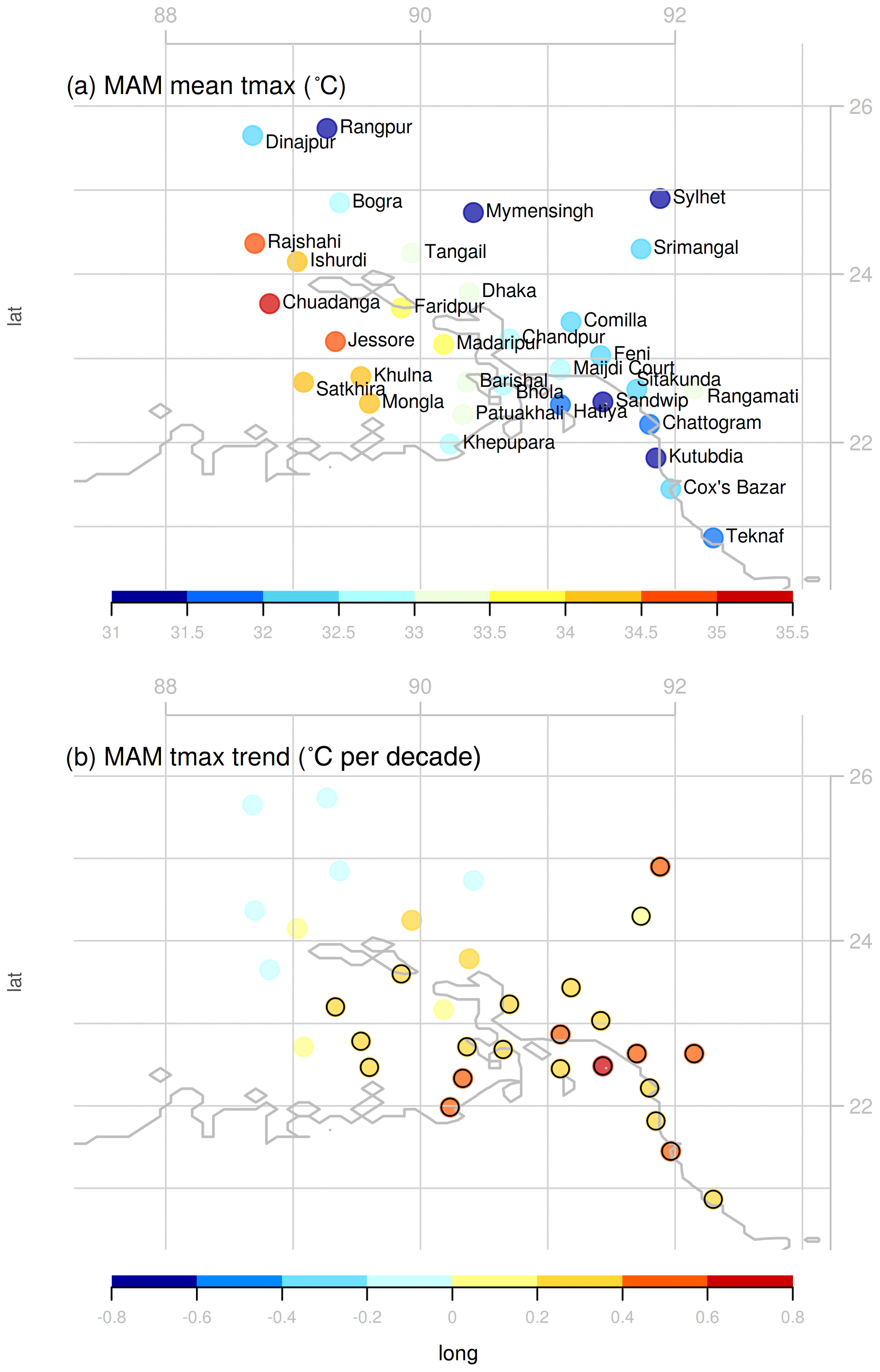
Figure 3(a) Pre-monsoon (March–May) seasonal mean of the daily maximum temperature at different stations in Bangladesh, and (b) the trend in daily maximum temperature, based on observations from 1981–2019. The black circles around the markers in (b) indicate that the trend is statistically significant at the 99 % level (p values < 0.01).
Due to the daily intense heating of the land surface over northwestern Bangladesh, low pressure systems tend to develop over Bihar, West Bengal of India and the adjoining northwestern part of Bangladesh. In the afternoons, moisture from the Bay of Bengal occasionally incurs to the low pressure system resulting in the formation of thunder clouds and severe thunderstorms. These severe thunderstorms are known as Nor'westers (“Kalbaishakhi” in Bengali) and they occur frequently at many places across Bangladesh in the pre-monsoon season. The Nor'westers are often accompanied by destructive squalls, thunder and heavy rainfall with hail. Flash floods typically occur in the northeastern part of Bangladesh due to heavy rainfall associated with severe thunderstorms, especially over northeastern parts of Bangladesh and adjoining northeastern states of India. Nevertheless, only 19 % of the total annual rainfall occurs in the pre-monsoon season.
The pre-monsoon season is also characterized by cyclogenesis in the Bay of Bengal. Some of the low pressure systems formed over the Bay of Bengal intensify into depressions which sometimes turn into storms and move initially northwestwards and subsequently recurve to the northeast towards the coast of Bangladesh and Myanmar (Khatun et al., 2016). Some of these storms become very severe at landfall along the Bangladeshi coast. They are occasionally associated with storm surges and may cause high casualties and damages.
2.1 Data description
Local observations of the daily maximum temperature from stations in Bangladesh were collected from the Bangladesh Meteorological Department (BMD). Only stations with at least 30 years of valid data in the calibration period 1981–2019 were retained. Further information about the observational stations are found in Table S1 of the Supplement.
The ERA5 data set (Hersbach et al., 2020; C3S, 2017), a global atmospheric reanalysis produced by the European Centre for Medium-Range Weather Forecasts (ECMWF), was used as predictor data to describe the pre-monsoon seasonal mean temperature over the domain 80–100∘ E/15–45∘ N.
Mean temperature GCM data from the CMIP5 ensemble were downloaded from the KNMI Climate Explorer (https://climexp.knmi.nl/start.cgi, last access: 21 January 2021) which provides monthly data regridded to a 2.5∘ resolution for the time period of 1900–2100. Three future pathways were considered: the high emission scenario RCP8.5 (Riahi et al., 2007), the medium emission scenario RCP4.5 in which the radiative forcing stabilizes shortly after 2100 (Clarke et al., 2007), and the more optimistic peak-and-decline scenario RCP2.6 (Van Vuuren et al., 2007). It should be noted that the ensemble size and climate models included differ between RCPs, as shown in Table S2.
2.2 Empirical-statistical downscaling method
The empirical-statistical downscaling approach used in this study involved deriving statistical relationships between the mean daily maximum temperature over the pre-monsoon season from station based observations in the period 1981–2019 and the large-scale mean temperature patterns as represented by the common EOFs of the ERA5 reanalysis and GCM simulations. In other words, we chose the downscaling “climate” approach here, focusing on the statistical characteristics of the daily maximum temperature.
A principal component analysis (PCA) was applied to the seasonally averaged observational data which decomposed the data into a set of spatial patterns, associated principle components (PC) describing their variation in time, and eigenvalues describing the relative weight of the various patterns. The first two leading PCs, which accounted for approximately 94 % (80 % for PC1 and 14 % for PC2) of the variability of the observed maximum temperature, were used as predictands.
A common EOF analysis, as proposed by Benestad (2001), was applied to the reanalysis and GCM maximum temperature data extracted for the domain 80–100∘ E/15–45∘ N to represent the large-scale predictors (Benestad et al., 2016). The GCM data (one simulation at a time, using the full period of available data 1850–2100) was combined with ERA5 reanalysis data for the period 1979–2019 along the time axis. EOF analysis was subsequently applied to the combined data set. This procedure decomposed the data into a set of spatial patterns and eigenvalues that were common to the reanalysis and GCM data, and principal components (PCs) for each pattern representing temporal variations where one part was associated with the reanalysis data and another part associated with the GCM data (Fig. 1). The part of the PCs associated with the reanalysis data were then used to calibrate a statistical model as follows:
where Y1 is the first leading PC of the predictand, X1, X2, …, X10 are the ten leading PCs of the predictor, and c0, c1, …, c10 are model coefficients obtained through multiple regression. Similar models were fitted for the second PC of the predictand. The number of predictor patterns was chosen because for all ensemble members, the ten leading common EOF patterns explain almost all (99 %–100 %) of the variance of the GCM simulation and reanalysis data.
A stepwise multiple regression was used to estimate model parameters, using predictand and predictor data from the calibration period 1981–2019. Only the part of the predictor PCs that represent the reanalysis were included in the regression. The number of predictors was reduced using the Akaike Information Criterion (AIC), a measure of model quality which takes both model performance and complexity into consideration in order to avoid overfitting (Akaike, 1974). In practise, this means that one or several of the coefficients c0, c1, …, c10 can be set to zero during model calibration. The statistical model was then applied to the predictor PCs associated with the GCM data to obtain future projections of the predictand PCs. Future estimates of the local maximum temperature could then be constructed from the projections of the predictand PCs combined with the corresponding spatial patterns and eigenvalues.
The procedure of common EOF analysis and stepwise multiple regression was repeated for each GCM simulation, but because the calculations were rather efficient they could nevertheless be applied to a large number of simulations (see Table S2 for a complete list of the included GCM simulations).
2.3 Validation
To evaluate the skill of the empirical-statistical models, a five-fold cross validation was applied in which the fitting process was repeated five times (Maraun et al., 2015), each time leaving one fifth of the predictor and predictand data out of the multiple regression (Wilks, 2011). Predictions were then made for the left out period and a cross validation score was calculated as the correlation (Pearson's r) between these independent predictions and the original principal components. The cross validation was performed for every regression model, i.e., for each PC and GCM simulation.
To assess how well the downscaled multi-model ensembles represent the past trends and interannual variability for each station, the observed seasonal mean maximum temperature in the period 1981–2019 was compared with statistical characteristics of the downscaled ensembles. The trend in the period 1981–2019 was calculated for the observed maximum temperature and for each downscaled ensemble member at all stations. To estimate the probability (ptrend) of seeing a maximum temperature trend of the observed strength given that the downscaled multi-model ensemble was a true representation of the distribution, the observed trend in the calibration period was compared with the probability density function (pdf) of a normal distribution (the “pnorm” function in R) with statistical characteristics (mean and standard deviation) given by maximum temperature trends of the downscaled ensemble members in the same period. To assess the representation of the interannual variability, the number of observed values outside of the 90 % confidence interval (CI) of the downscaled ensemble was counted and the probability of the outcome (pCI) was calculated using a binomial pdf (the “pbinom” function in R). On average, 10 % of values are expected to fall outside of the 90 % CI, and a much higher (lower) number of values outside of this range suggests that the downscaled ensemble may be underestimating (overestimating) the interannual variability. The results of the ensemble validation are summarised in a target plot with ptrend on the x axis and pCI on the y axis (see Fig. 6).
2.4 Analysis software
The analysis was carried out within the R-environment using the “esd” package (Benestad et al., 2015b) to analyze and visualize the data and perform the statistical downscaling. The “esd” package has a wide range of functionalities, including methods for reading and processing data, generating various infographics, and performing statistical analysis (e.g., calculating empirical orthogonal functions, principal component analysis, and empirical-statistical downscaling) and is suitable for processing results from global climate models.
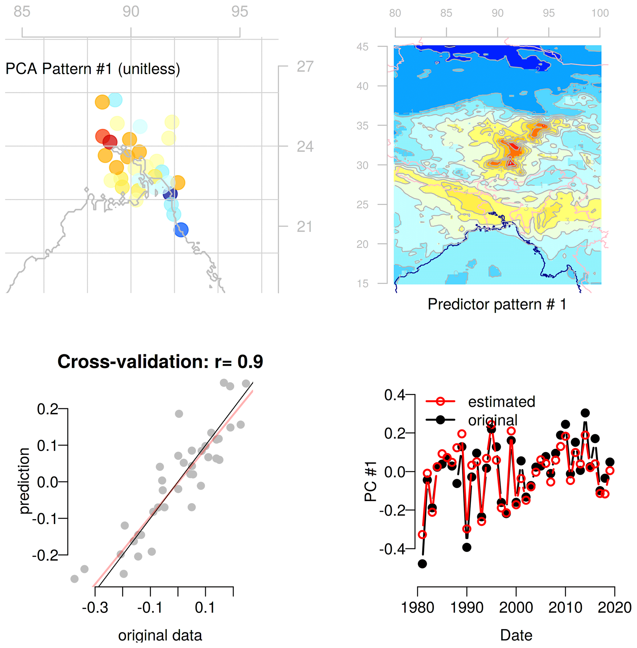
Figure 4Evaluation of the statistical downscaling of the maximum temperature in the pre-monsoon season (March–May) for the leading principal component of the predictand (PC1). The four panels show (a) the spatial pattern associated with PC1, (b) the predictor pattern associated with PC1, i.e., the spatial co-variance structure of the ERA5 reanalysis data used as predictor (the pre-monsoon seasonal mean temperature in the domain 80–100∘ E/15–45∘ N) and the leading principal component of the local temperature observations in the calibration period 1981–2019, (c) a cross-validation comparing the original PC1 of the predictand and the corresponding estimated values obtained by empirical-statistical downscaling, and (d) time series of the estimated and original PC1 of the predictand.
3.1 Past climate change in Bangladesh
Based on the observations, the average daily maximum temperature in Bangladesh in the pre-monsoon season has changed by between −0.04 and +0.67 ∘C per decade over the period 1981–2019, depending on the station (Fig. 3; Table S1). The average temperature increase over all stations is +0.30 ∘C per decade. While the average observed maximum temperature during the period was highest in the west (Fig. 3a), the strongest change occurred in the east (Fig. 3b), which means that there has been a decrease in the east–west temperature gradient over the last decades. The warming observed in the central and eastern stations was statistically significant (p<0.01 based on a student's t-test) while the trends in the west were not (Fig. 3b).
3.2 Validation of the statistical downscaling
An evaluation of the statistical downscaling models is shown in Figs. 4 and 5. The cross-validated correlation between the first (PC1) and second (PC2) principal components of the maximum temperature and the corresponding PCs estimated based on empirical-statistical downscaling were 0.90 and 0.61, respectively, when using only the reanalysis as predictor data (both statistically significant with p values lower than 0.01). A separate regression model was fitted for each reanalysis-GCM simulation combination and the cross validation was also repeated for all ensemble members. For PC1, the cross validation correlation score was between 0.82 and 0.92, in all cases statistically significant with p values < 10−9. For PC2, the cross validation ranged between 0.11 and 0.69, and only in 63 % of the ensemble members statistically significant at the 99 % level (i.e., p<0.01). An attempt was made to downscale PC3 and PC4 too, but the cross-validation indicated that the esd models had little predictive power for these PCs, with lower correlation scores (0.36 and 0.13, respectively when using only the reanalysis as predictor) that were not statistically significant (the 95 percent confidence intervals of the correlation scores spanned negative and positive values). PC3 and PC4 are thus excluded from the future projections of maximum temperature.
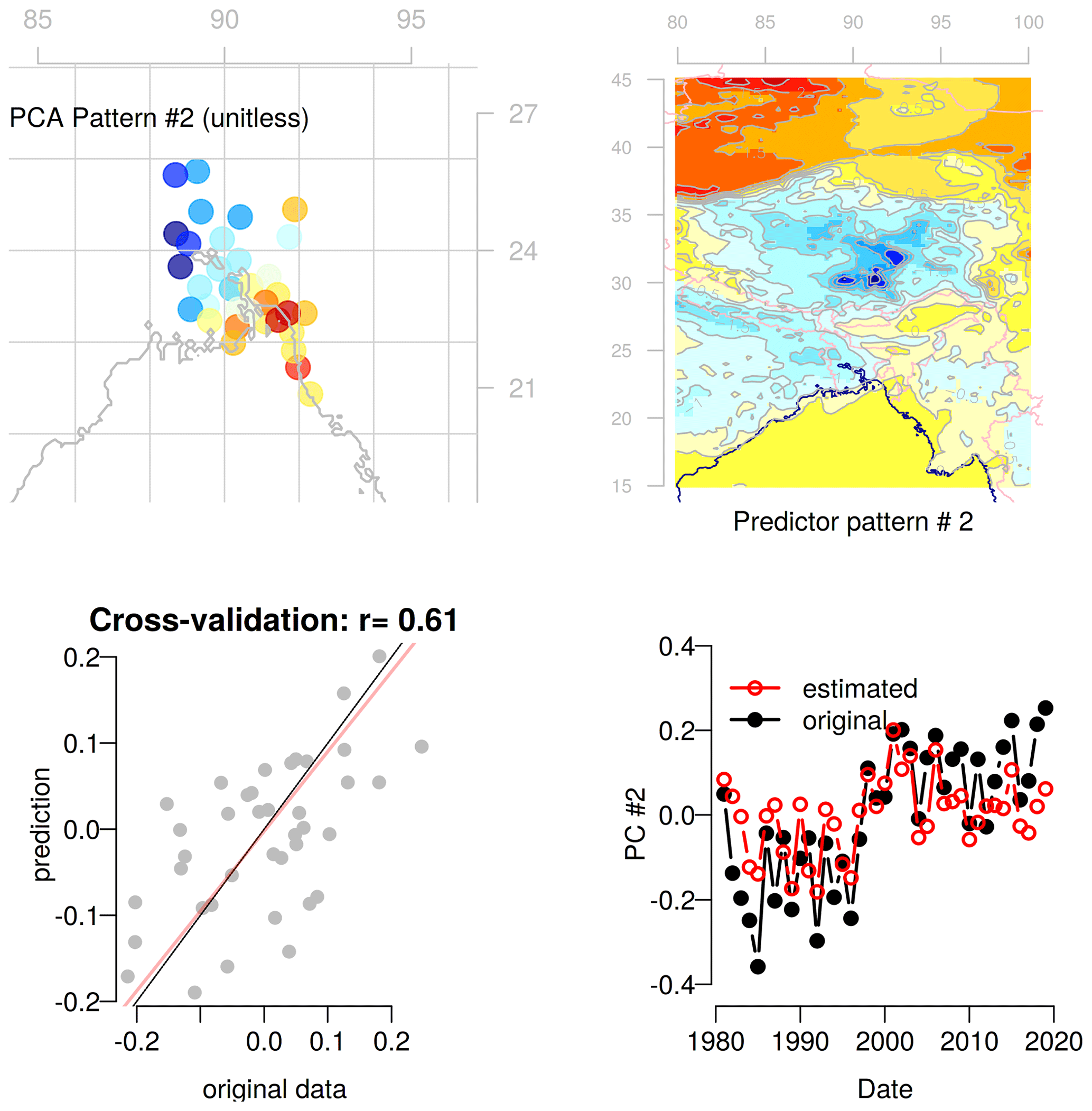
Figure 5Evaluation of the statistical downscaling of the maximum temperature in the pre-monsoon season (March–May) for the second leading principal component of the predictand (PC2). Details like in Fig. 4.
As further validation, the statistical characteristics of the downscaled ensembles were compared to the observed maximum temperature as described in Sect. 2.3. The results presented in Fig. 6 suggest a spatial pattern where the downscaled ensemble tends to underestimate both the trend and interannual variability in the south-east, but gives a better representation of the observed statistical characteristics in the central and western part of Bangladesh. Figure 6 displays results only for RCP4.5, but the other emission scenarios (not included here) showed qualitatively similar results.
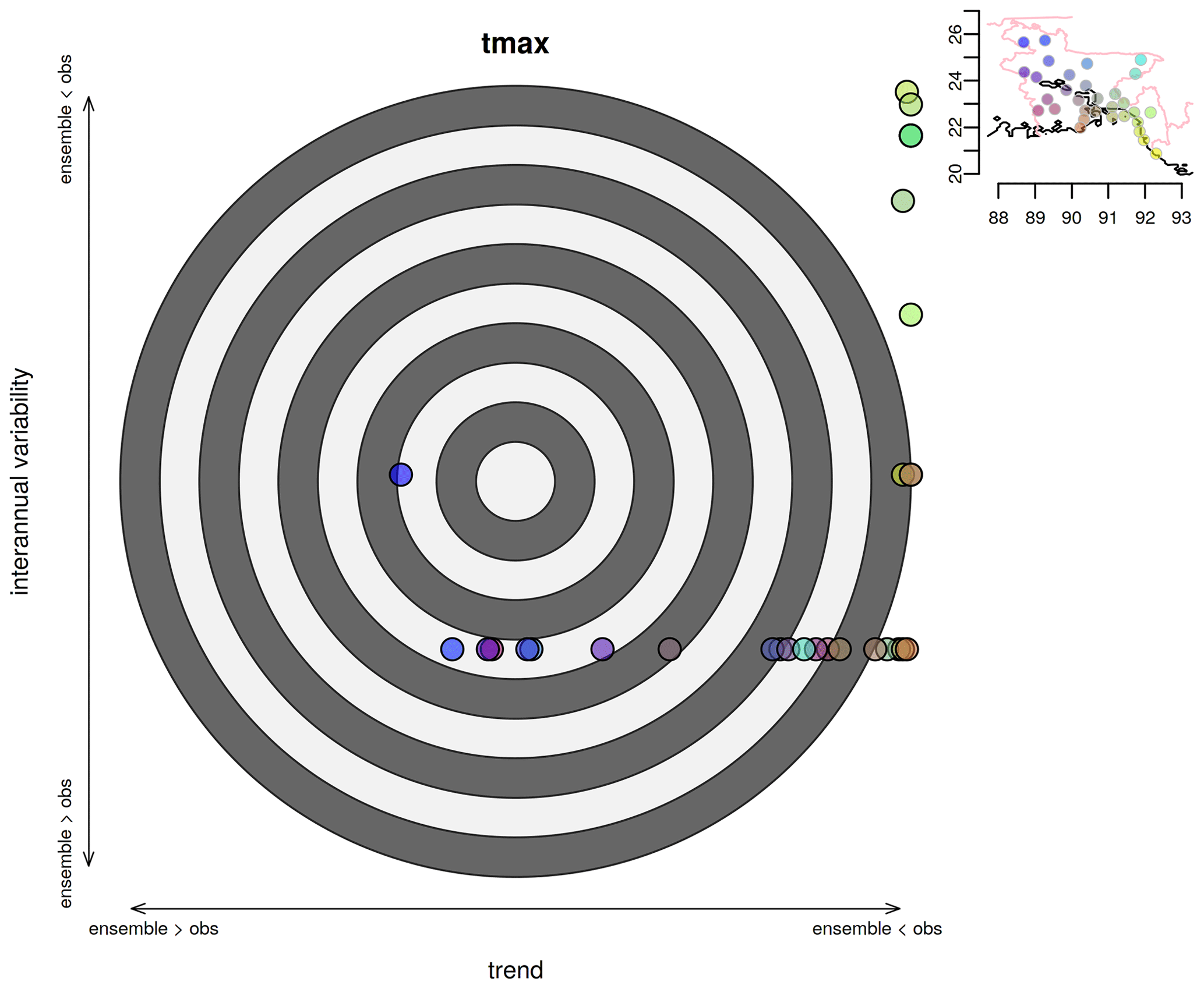
Figure 6Evaluation of the ensemble of statistically downscaled maximum temperature in the pre-monsoon season (March–May) based on emission scenario RCP4.5 and observations in the period 1981–2019. Each point represents a station and the colors show the geographical location as seen in the map in the upper right corner. The x axis shows the probability of the observed trend given a distribution with the statistical characteristics (mean and standard deviation) of the trends of the downscaled ensemble. Values far to the right (left) indicate that the downscaled ensemble is underestimating (overestimating) the trend. The y axis shows the probability of finding the observed number of values outside of the downscaled ensemble 90 % confidence interval, which is taken as a measure of how well the ensemble represents the interannual variability. Values towards the top (bottom) suggest that the downscaled ensemble underestimates (overestimates) the interannual variability.
3.3 Future projections of pre-monsoon maximum temperature
Figure 6 shows an example of downscaled ensembles of climate projections for the station Dhaka for the different emission scenarios (RCP2.6, RCP4.5 and RCP8.5). The results for all stations are summarized in Table 1, which includes the ensemble mean of the change in the maximum temperature of the pre-monsoon season for two periods: the near future (2021–2050) and the far future (2071–2100) relative to the base period 1981–2010. Figure 8 additionally displays the ensemble mean of the projected temperature change at the various stations on a map. The ensemble mean of the downscaled projections indicated an increase in the maximum temperature in Dhaka by +0.8 ∘C for the near future and +1.0 ∘C for the far future assuming RCP2.6. For RCP4.5, the estimated temperature rise in Dhaka is +0.9 and +1.6 ∘C for the near and far future, respectively. The most severe scenario, RCP8.5, suggested an increase of +1.0 ∘C for the near future which is intensified for the far future reaching up to +3.0 ∘C. The projected change for Dhaka is slightly higher than the average increase in maximum temperature over all stations in Bangladesh.
Table 1Ensemble mean change in maximum temperature (unit: ∘C) for the pre-monsoon season (March-May) in Bangladesh for the near future (2021–2050) and the far future (2071–2100) compared to the base period 1981–2010. Projected changes are shown for three emission scenarios: RCP2.6, RCP4.5, and RCP8.5.

The estimated ensemble mean warming in the near future is independent of the chosen scenario (+0.7 ∘C for RCP2.6, RCP4.5, and RCP8.5), but for the far future the different scenarios have a larger impact on the results, which show an ensemble mean warming of +0.8, +1.2 and +2.2 ∘C for RCP2.6, RCP4.5, and RCP8.5, respectively. The highest projected ensemble mean warming at individual stations for RCP4.5 was +1.0 ∘C for the near future and +1.4 ∘C for the far future (both at the station Ishurdi). For the most severe emission scenario, RCP8.5, the strongest projected warming was +1.2 and +3.2 ∘C for the near and far future, respectively (also at Ishurdi).
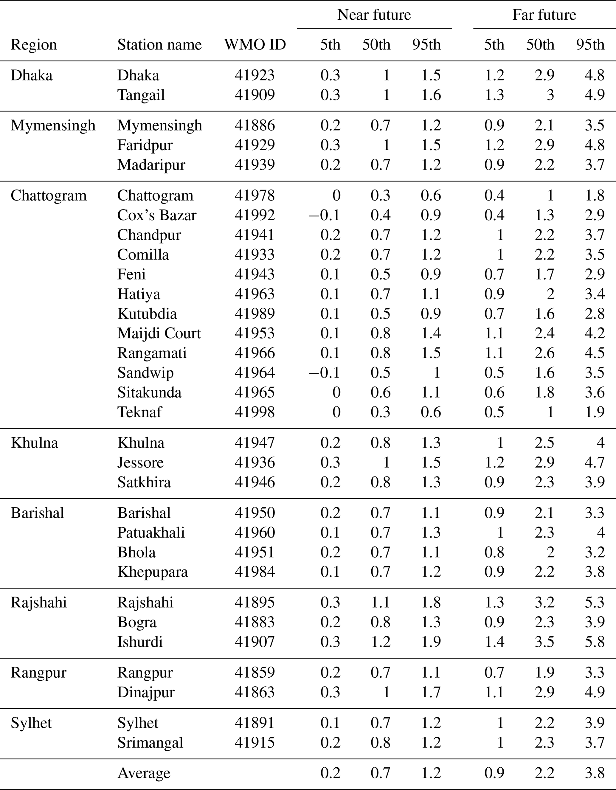
Tables 2–4 display ensemble statistics (5th, 50th and 95th percentiles) of the projected change in maximum temperature relative to the base period 1981–2010 for the emission scenarios RCP2.6, RCP4.5, and RCP8.5, respectively. The ensemble spread can be interpreted as representative of the internal climate variability as well as model differences. The average 5th percentile of projected temperature change over all stations in Bangladesh for the far future (2071–2100) assuming RCP2.6 (Table 2) is +0.1 ∘C, indicating that 5 % of the included projections show little change or even a temperature decrease compared to the base period (1981–2010). The corresponding 50th and 95th percentiles of temperature change is +0.8 and +1.6 ∘C, respectively, indicating that 50 % observations are showing changes of temperature of +0.8 ∘C or more but only 5 % showed a warming of +1.6 ∘C or higher. For RCP4.5 (Table 3), the 5th, 50th and 95th percentiles of the projected temperature changes averaged over all stations are +0.4, +1.2 and +2.3 ∘C from the base period to the far future. The corresponding ensemble statistics of maximum temperature change for RCP8.5 describe an even stronger warming, with station average 5th, 50th and 95th percentiles of +0.9, +2.2 and +3.8 ∘C, respectively (Table 4).
Table 2The 5th, 50th and 95th percentile values of projected changes in maximum temperature (unit: ∘C) in Bangladesh for the near future (2021–2050) and far future (2071–2100) relative to the 1981–2010 period for RCP2.6.
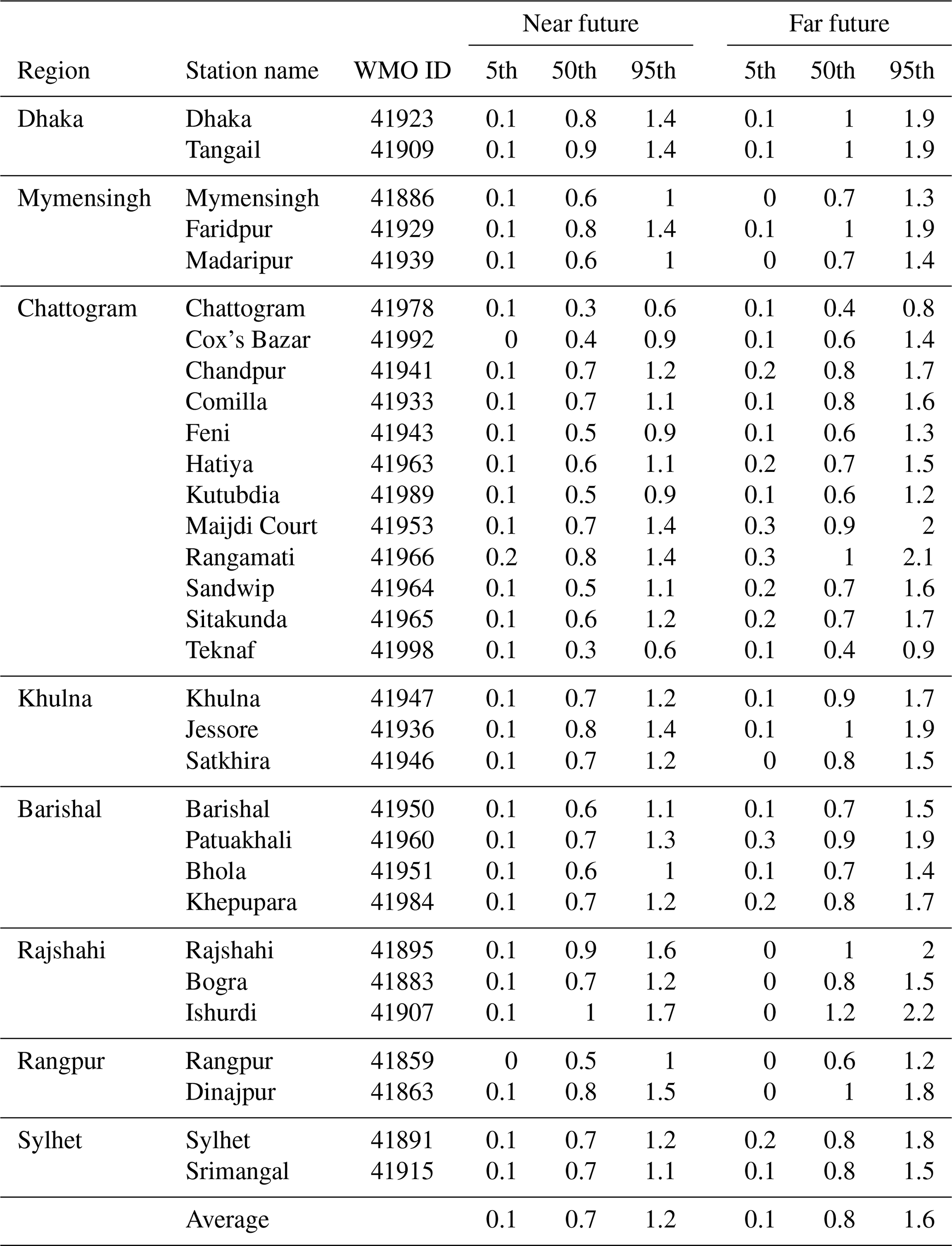
Table 3The 5th, 50th and 95th percentile values of projected changes in maximum temperature (unit: ∘C) in Bangladesh for the near future (2021–2050) and far future (2071–2100) relative to the 1981–2010 period for RCP4.5.
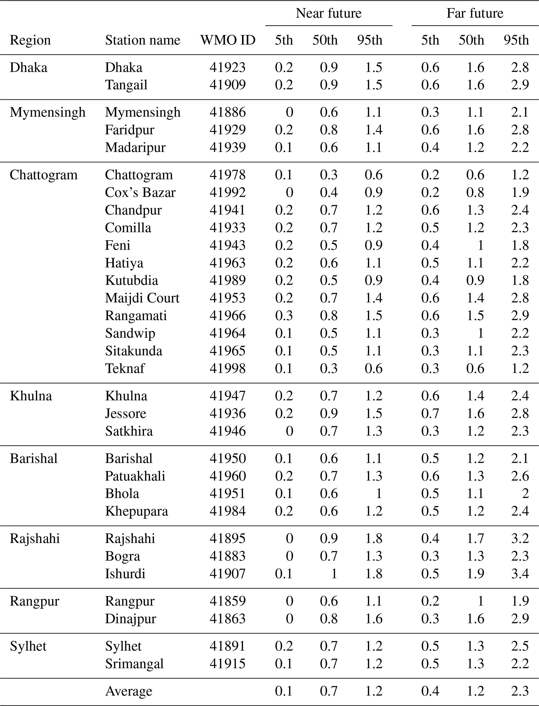
Table 4The 5th, 50th and 95th percentile values of projected changes in maximum temperature (unit: ∘C) in Bangladesh for the near future (2021–2050) and far future (2071–2100) relative to the 1981–2010 period for RCP8.5.
The three emission scenarios considered in this study lead to an increase in the expected seasonal mean maximum temperature in the future in Bangladesh. The low-emission scenario RCP2.6 describes a future in which CO2 emissions remain constant until the early 21st century and become negative by the end of the century. As a result, the radiative forcing reaches a value of around 3.1 W m−2 by mid-century but returns to 2.6 W m−2 by 2100. Based on this scenario, our results suggest that the average pre-monsoon maximum temperature over meteorological sites in Bangladesh is likely to increase in the near future and then increase only slightly till the end of the 21st century. Following the low-to-moderate emission scenario RCP4.5 or the high-emission scenario RCP8.5, the average projected warming in Bangladesh in the near-future is similar to the warming under RCP2.6, but continuing into the far future the warming is considerably higher, reaching around +1.2 and +2.2 ∘C for RCP4.5 and RCP8.5, respectively. Similarly to the RCP2.6, the intermediate path RCP4.5, is characterised by a peak-and-decline scenario in which emissions are considerably reduced after 2050 leading to a stabilization of radiative forcing toward the end of the 21st century. The continued increase of the projected maximum temperature following both RCP2.6 and RCP4.5 demonstrates the inertia of the climate system and the lag in the response of temperature to greenhouse gas emissions and radiative forcing.
The projected increase in maximum temperature in the already hot pre-monsoon season indicates that there will likely be an increase in the frequency and intensity of heat waves in Bangladesh. In the southwest and northwest regions, the maximum pre-monsoon temperature is already very high (Figs. 2 and 3, Table S1) and severe heat waves are already a common occurrence, and an increase of several degrees as our estimates suggest (see the regions Khulna, Rajshahi and Rangpur in Tables 1–4), could be detrimental to the life and health of people living in these areas.
One important motivation behind the ESD method applied in this paper was to make use of the large scales that the models are able to reproduce realistically to say something about local changes. All GCMs have a minimum skillful scale which means that their individual grid-box values are not a good representation of the area they represent in the real world (through design and because computers work with discrete numbers). The use of common EOF analysis makes it possible to identify common spatial patterns in reanalysis and GCM data on a scale that is well represented by climate models.
A potential limitation of the statistical downscaling method presented here is that the predictor-predictand relationship may not be stationary, i.e., the statistical model may not be applicable to future periods. The stationarity assumption is central to empirical-statistical downscaling but difficult to validate, especially without access to long observational records. Here, the local pre-monsoon maximum temperature was downscaled from the mean temperature over the domain 80–100∘ E/15–45∘ N. There are circumstances that could change the predictor–predictand relationship in a period of climate change. For example, the local temperature response to large-scale temperature patterns could be influenced by changes in precipitation patterns, cyclonic activity and the timing of the monsoon. One way to address this could be to incorporate additional predictor variables that describe other aspects of the climate.
While observations showed a stronger pre-monsoon warming in the east compared to the west in the past (1981–2019), which reduced the east–west temperature gradient in this period (Fig. 2), there was less of an obvious spatial pattern in the projected maximum temperature (Fig. 7). A simple correlation analysis indicates that there was no statistically significant correlation between the longitude/latitude and the rate of projected warming.
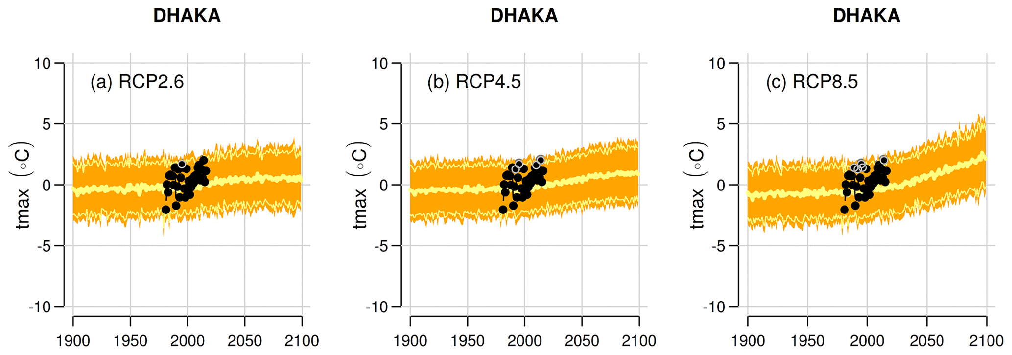
Figure 7Downscaled projections of the maximum temperature in the pre-monsoon season (March–May) in Dhaka for emission scenarios RCP2.6, RCP4.5, and RCP8.5. The figures show the change relative to the period 1981–2010. The shaded area indicates one standard deviation from the mean based on the included GCM simulations for each experiment.

Figure 8Ensemble mean of the downscaled projections of the maximum temperature in the pre-monsoon season (March–May) for stations in Bangladesh. The panels show the projected change in maximum temperature from the reference period (1981–2010) to the near future (2021–2050, shown in a–c) and far future (2071–2100, shown in d–f) assuming emission scenarios RCP2.6 (a, e), RCP4.5 (b, f), and RCP8.5 (c, g). The range of the color scale (0–+2 ∘C) does not span the full range of projected temperature changes for the far future assuming RCP8.5 (see Tables 1 and 4).
In the current analysis, only the two leading predictand PCs were downscaled. This was done because higher order PCs contained little information about the large-scale climate structure and thus could not be robustly downscaled. An attempt was made to downscale the third and fourth PCs but cross-validation indicated that the statistical models had little to no predictive power. This makes sense as the leading PCs represented coherent temperature anomalies on larger scales which are more likely connected to large-scale forcing. Since the first two PCs stand for a majority of the observed maximum temperature variability and the observed trends, this should be enough to represent the relevant variations and trends, assuming sufficiently skillful regression models for PC1 and PC2.
PC1 represents 80 % of the variability of the observed pre-monsoon maximum temperature in Bangladesh and partly contains the trend in the reference period 1981–2019 (Fig. 4). However, the spatial pattern in the observed temperature trend, which shows a stronger warming in eastern and south-eastern Bangladesh compared to the western part of the country (Fig. 3), is contained within PC2 (Fig. 5). At the stations with strongest trends, 30 %–60 % of the trend is represented by predictand PC2. The regression model, which was trained on detrended data, slightly underestimated the long term trend in PC1 indicating that there is only a slight non-stationarity problem. This is more pronounced in PC2, which also has a poorer performance and represents a smaller fraction of the covariance. Since the downscaling models of PC2 are not as skillful as the models for PC1 (see cross-validation scores in Sect. 3.2 and Figs. 4c and 5c), the downscaling models fail to reproduce the observed gradient in the maximum temperature trend in the calibration period (Fig. 8). Further validation by inspection of the downscaled ensemble (Fig. 6) suggested that the downscaling reproduced the statistical characteristics of the observed climate well in central and western Bangladesh but in the east and south-east, which is the region with the strongest warming in the past (Fig. 3b), the downscaling tends to underestimate the trend and interannual variability at some stations.
A possible explanation why the large-scale temperature is not a perfect predictor of PC2 could be that the observed spatial differences in warming are related to changes in precipitation patterns or other environmental circumstances that are not captured by the chosen predictor (the mean temperature). A preliminary analysis where the pre-monsoon maximum temperature was downscaled with alternative predictor variables from the ERA5 and CMIP5 data sets indicated that the mean Sea Level Pressure (SLP) or precipitation are better predictors than the mean temperature for PC2, but not as good for PC1 (not shown here). The downscaling method could be improved by the inclusion of multiple predictors, using multivariate EOFs and/or allowing different predictor variables for different predictor PCs. If the spatial patterns of pre-monsoon precipitation and drought change in the coming decade, as projected by Khan et al. (2020), a downscaling strategy allowing multiple climate drivers may have a better chance of representing the effect of these changes on the temperature.
To evaluate the influence of the predictor, the downscaling was performed with a variable number of predictor patterns. The cross validation scores indicated that the leading 8-10 predictor patterns should be included to achieve the best downscaling models, but including higher order patterns had little effect on the outcome, both in terms of cross validation, reproducing the present climate, and for the projected temperature change. A closer look at the common EOFs showed that 99 %–100 % of the variability was contained within the leading 8–10 predictor patterns for all GCM-reanalysis combinations, which explains why higher order modes of variability added no skill. These results suggest that the stepwise model selection should be applied to all predictor patterns that hold relevant information (e.g., considering all modes with an explained variance of 1 % or higher).
There is a subtle difference between the way that the principal component analysis of the predictand and the EOF analysis of the predictor is used in the downscaling method. For the predictor, only the eigenvectors representing the temporal variations of the predictor patterns are used in the regression models. This means that the predictor patterns are not explicitly weighted by their relative importance. The stepwise model selection will instead determine which patterns are important, and since including additional parameters in the linear regression costs little time and computational resources, we can include all potentially relevant predictor patterns. For the predictand on the other hand, the downscaled predictand PCs are combined with the corresponding eigenvalues and spatial eigenvectors to obtain temperature projections. The leading PCs are thus given larger weight by its eigenvalue than higher order PCs. Every additional predictand PC included requires another regression for every GCM simulation, which can add significant computation time. Downscaling higher order predictand PCs can therefore be a waste of time and computational resources if they have low eigenvalues and their regression models have little predictive power.
We conclude that future CO2 emissions are expected to have severe consequences for the hottest season in Bangladesh in terms of significant warming in the whole country. All emission scenarios indicate an increasing pre-monsoon maximum temperature in Bangladesh, but while RCP2.6 shows the temperature plateauing mid-century, the average increase is 2 times higher in the far future compared to the near future assuming RCP4.5, and 3 times higher assuming RCP8.5. This illustrates that while warming may be unavoidable, there are still opportunities to limit the severity of climate change in the future.
The code used to perform the analysis has been made available at Figshare: https://doi.org/10.6084/m9.figshare.14844984.v2 (Parding and Rashid, 2021).
The temperature observations from stations in Bangladesh, provided by the Bangladesh Meteorological Department, are not publicly available. The ERA5 Fifth generation of ECMWF atmospheric reanalyses of the global climate are available for download from C3S Copernicus Climate Change Service (https://doi.org/10.24381/cds.f17050d7, Hersbach et al., 2019). The global climate model data from the Coupled Model Intercomparison Project Phase 5 (CMIP5) were downloaded from the KNMI Climate Explorer (https://climexp.knmi.nl/, WMO and KNMI, 2021).
The supplement related to this article is available online at: https://doi.org/10.5194/asr-18-99-2021-supplement.
MBR and KMP prepared the manuscript with major contributions from RB and AM, and further contributions from SSH, MAM, and HOH. MBR and KMP performed the empirical-statistical downscaling and additional analysis. REB, AM and KMP developed the software used to perform the statistical analysis. All authors contributed to the manuscript.
The authors declare that they have no conflict of interest.
This article is part of the special issue “Applied Meteorology and Climatology Proceedings 2020: contributions in the pandemic year”.
This study was partly funded by NORAD, and supported by Bangladesh Meteorological Department (BMD) and the Norwegian Meteorological Institute (MET Norway). The authors would like to thank the anonymous reviewers whose constructive feedback helped clarify and improve this manuscript. We acknowledge the World Climate Research Programme, which coordinated the CMIP5 project, the climate modeling groups that produced the climate model output, and the Royal Netherlands Meteorological Institute (KNMI) and WMO for making data available through the KNMI climate explorer, as well as ECMWF and the Copernicus Climate Change Service (C3S) Climate Data Store (CDS) for providing the ERA5 reanalysis data. The authors also gratefully acknowledge BMD for providing observational data.
This research has been supported by the Direktoratet for Utviklingssamarbeid (grant no. RAS-2820 RAS-17/0009 (Meteorological services in Bangladesh, Myanmar and Vietnam 2017–2019)).
This paper was edited by Andreas Fischer and reviewed by three anonymous referees.
Akaike, H.: A new look at the statistical model identification, IEEE T. Automat. Control, 19, 716–723, https://doi.org/10.1109/TAC.1974.1100705, 1974.
Alamgir, M., Ahmed, K., Homsi, R., Dewan, A., Wang, J.-J., and Shahid, S.: Downscaling and Projection of Spatiotemporal Changes in Temperature of Bangladesh, Earth Syst. Environ., 3, 381–398, https://doi.org/10.1007/s41748-019-00121-0, 2019.
Barnett, T. P.: Comparison of Near-Surface Air Temperature Variability in 11 Coupled Global Climate Models, J. Climate, 12, 511–518, 1999.
Benestad, R. E.: A Comparison between Two Empirical Downscaling Strategies. Int. J. Climatol., 21, 1645–1668, https://doi.org/10.1002/joc.703, 2001.
Benestad, R. E.: Downscaling Climate Information, Oxford Research Encyclopedia, Oxford, https://doi.org/10.1093/acrefore/9780190228620.013.27, 2016.
Benestad, R. E., Hanssen-Bauer, I., and Chen, D.: Empirical Statistical Downscaling, World Scientific Publishing Company, New Jersey, London, 2009.
Benestad, R. E.: A New Global Set of Downscaled Temperature Scenarios, J. Climate, 24, 2080–2098, 2011.
Benestad, R. E., Chen, D., Mezghani, A., Fan, L., and Parding, K. M.: On Using Principal Components to Represent Stations in Empirical-Statistical Downscaling, Tellus A, 67, 28326, https://doi.org/10.3402/tellusa.v67.28326, 2015a.
Benestad, R. E., Mezghani, A., and Parding, K. M.: The Empirical-Statistical Downscaling Tool & Its Visualisation Capabilities, Met Report 11/2015, Norwegian Meteorological Institute, Oslo, Norway, 2015b.
Benestad, R. E., Parding, K. M., Isaksen, K., and Mezghani, A.: Climate Change and Projections for the Barents Region: What Is Expected to Change and What Will Stay the Same?, Environ. Res. Lett., 11, 054017, https://doi.org/10.1088/1748-9326/11/5/054017, 2016.
Clarke, L. E., Edmonds, J. A., Jacoby, H. D., Pitcher, H., Reilly, J. M., and Richels, R.: Scenarios of Greenhouse Gas Emissions and Atmospheric Concentrations, Sub-Report 2.1a of Synthesis and Assessment Product 2.1, Climate Change Science Program and the Subcommittee on Global Change Research, Department of Energy, Office of Biological & Environmental Research, Washington, DC, 2007.
C3S – Copernicus Climate Change Service: ERA5: Fifth generation of ECMWF atmospheric reanalyses of the global climate, Copernicus Climate Change Service Climate Data Store (CDS), available at: https://cds.climate.copernicus.eu/cdsapp#!/home (last access: 20 January 2021), 2017.
Flury, B.: Common Principal Components & Related Multivariate Models, John Wiley & Sons, Inc., USA, ISBN 0471634271, 1988.
Giorgi, F. and Gutowski Jr., W. J.: Regional Dynamical Downscaling and the CORDEX Initiative, Annu. Rev. Environ. Resour., 40, 467–490, https://doi.org/10.1146/annurev-environ-102014-021217, 2015.
Glahn, H. R.,and Lowry, D. A.: The Use of Model Output Statistics (MOS) in Objective Weather Forecasting, J. Appl. Meteorol., 11, 1203–1211, 1972.
Gudmundsson, L., Bremnes, J. B., Haugen, J. E., and Engen-Skaugen, T.: Technical Note: Downscaling RCM precipitation to the station scale using statistical transformations – a comparison of methods, Hydrol. Earth Syst. Sci., 16, 3383–3390, https://doi.org/10.5194/hess-16-3383-2012, 2012.
Gutjahr, O. and Heinemann, G.: Comparing precipitation bias correction methods for high-resolution regional climate simulations using COSMO-CLM, Theor. Appl. Climatol., 114, 511–529, 2013.
Gutman, E. D., Rasmussen, R. M., Liu, C., Ikeda, K., Gochis, D. J., Clark, M. P., Dudhia, J., and Thompson, G.: A Comparison of Statistical and Dynamical Downscaling of Winter Precipitation over Complex Terrain, J. Climate, 30, 262–281, https://doi.org/10.1175/2011JCLI4109.1, 2012.
Hersbach, H., Bell, B., Berrisford, P., Biavati, G., Horányi, A., Muñoz Sabater, J., Nicolas, J., Peubey, C., Radu, R., Rozum, I., Schepers, D., Simmons, A., Soci, C., Dee, D., and Thépaut, J.-N.: ERA5 monthly averaged data on single levels from 1979 to present, Copernicus Climate Change Service (C3S) Climate Data Store (CDS), https://doi.org/10.24381/cds.f17050d7, 2019.
Hersbach, H., Bell, B., Berrisford, P., Hirahara, S., Horányi, A., Muñoz-Sabater, J., Nicolas, J., Peubey, C., Radu, R., Schepers, D., Simmons, A., Soci, C., Abdalla, S., Abellan, X., Balsamo, G., Bechtold, P., Biavati, G., Bidlot, J., Bonavita, M., De Chiara, G., Dahlgren, P., Dee, D., Diamantakis, M., Dragani, R., Flemming, J., Forbes, R., Fuentes, M., Geer, A., Haimberger, L., Healy, S., Hogan, R. J., Hólm, E., Janisková, M., Keeley, S., Laloyaux, P., Lopez, P., Lupu, C., Radnoti, G., de Rosnay, P., Rozum, I., Vamborg, F., Villaume, S., and Thépaut, J.-N.: The ERA5 global reanalysis, Q. J. Roy. Meteorol. Soc., 146, 1999–2049, https://doi.org/10.1002/qj.3803, 2020.
Hewitson, B., Daron, J., Crane, R., Zermoglio, M., and Jack, C.: Interrogating empirical statistical downscaling, Climatic Change, 122, 539–554, 2014.
Khan, J. U., Islam, A. K. M. S., Das, M. K., Mohammed, K., Bala, S., Sujit, K., and Islam, G. M. T.: Future changes in meteorological drought characteristics over Bangladesh projected by the CMIP5 multi-model ensemble, Climatic Change, 162, 667–685, https://doi.org/10.1007/s10584-020-02832-0, 2020.
Khatun, M. A., Rashid, M. B., and Hygen, H. O.: Climate of Bangladesh, Met Report 08/2016, Norwegian Meteorological Institute, Oslo, Norway, 2016.
Kjellström, E., Bärring, L., Jacob, D., Jones, R., Lenderink, G., and Schär, C.: Modelling daily temperature extremes: recent climate and future changes over Europe, Climatic Change, 81, 249–265, https://doi.org/10.1007/s10584-006-9220-5, 2007.
Liu, J., Yuan, D., Zhang, L., Zou, X., and Song, X., Comparison of Three Statistical Downscaling Methods and Ensemble Downscaling Method Based on Bayesian Model Averaging in Upper Hanjiang River Basin, China, Adv. Meteorol., 2016, 7463963, https://doi.org/10.1155/2016/7463963, 2016.
Maraun, D.: Bias Correction, Quantile Mapping, and Downscaling: Revisiting the Inflation Issue, J. Climate, 26, 2137–2143, https://doi.org/10.1175/JCLI-D-12-00821.1, 2013.
Maraun, D. and Widmann, M.: Statistical Downscaling and Bias Correction for Climate Research, Cambridge University Press, Cambridge, https://doi.org/10.1017/9781107588783, 2018.
Maraun, D., Widmann, M., Gutiérrez, J. M., Kotlarski, S., Chandler, R. E., Hertig, E., Wibig, J., Huth, R., and Wilcke, R. A. I.: VALUE: A framework to validate downscaling approaches for climate change studies, Earth's Future, 3, 1–14, https://doi.org/10.1002/2014EF000259, 2015.
Mezghani, A., Dobler, A., Benestead, R. E., Haugen, J. E., and Parding, K. M.: Subsampling Impact on the Climate Change Signal over Poland Based on Simulations from Statistical and Dynamical Downscaling, J. Appl. Meteorol. Clim., 58, 1061–1078, 2019.
Mishra, V.: Climatic uncertainty in Himalayan water towers, J. Geophys. Res.-Atmos., 120, 2689–2705, 2015.
Nakicenovic, N., Alcamo, J., Grubler, A., Riahi, K., Roehrl, R. A., Rogner, H.-H., and Victor, N.: Special Report on Emissions Scenarios (SRES), in: A Special Report of Working Group III of the Intergovernmental Panel on Climate Change, Cambridge University Press, Cambridge, ISBN 0-521-80493-0, 2000.
Nury, A. H. and Alam, J. B.: Performance Study of Global Circulation Model HADCM3 Using SDSM for Temperature and Rainfall in North-Eastern Bangladesh, J. Scient. Res., 6, 87–96, https://doi.org/10.3329/jsr.v6i1.16511, 2013.
OECD: Development and climate change in Bangladesh: focus on coastal flooding and the Sundarbans, in: Organization for economic co-operation and development (OECD) report COM/ENV/EPOC/DCD/DAC (2003)3/FINAL, edited by: Agrawala, S., Ota, T., and Ahmed, A. U., Paris, France, available at: http://www.oecd.org/env/cc/21055658.pdf (last access: 21 June 2021), 2003.
Parding, K. and Rashid, M. B.: Code for empirical-statistical downscaling analysis, Figshare, https://doi.org/10.6084/m9.figshare.14844984.v2, 2021.
Pour, S. H., Shahid, S., Chung, E.-S., and Wang, X.-J.: Model output statistics downscaling using support vector machine for the projection of spatial and temporal changes in rainfall of Bangladesh, Atmos. Res., 213, 149–162, https://doi.org/10.1016/j.atmosres.2018.06.006, 2018.
Rahaman, A. Z., Khan, M. F. A., Aktar, N., Al Hossain, B. T., Akand, K., and Noor, F.: Climate Change Scenarios of Bangladesh Using Statistical Downscaling Model (SDSM), in: 5th International Conference on Water & Flood Management, 6–8 March 2015, Bangladesh University of Engineering and Technology, Bangladesh, 2015.
Rahman, M. M., Islam, M. N., Ahmed, A. U., and Georgi, F.: Rainfall and temperature scenarios for Bangladesh for the middle of 21st century using RegCM, J. Earth Syst. Sci., 121, 287–295, https://doi.org/10.1007/s12040-012-0159-9, 2012.
Riahi, K., Grübler, A., and Nakicenovic, N.: Scenarios of Long-Term Socio-Economic and Environmental Development under Climate Stabilization, Technol. Forecast. Social Change, 74, 887–935, https://doi.org/10.1016/j.techfore.2006.05.026, 2007.
Rummukainen, M.: State-of-the-art with regional climate models, WIREs Clim. Change, 1, 82–96, https://doi.org/10.1002/wcc.8, 2010.
Sanjay, J., Krishnan, R., Shrestha, A. B., Rajbhandari, R., and Ren, G.-Y.: Downscaled climate change projections for the Hindu Kush Himalayan region using CORDEX South Asia regional climate models, Adv. Clim. Change Res., 8, 20178, https://doi.org/10.1016/j.accre.2017.08.003, 2017.
Shourav, S. A., Mohsenipour, M., Alamgir, M., Hadipour, S., and Ismail, T.: Historical Trends and Future Projections of Climate at Dhaka City of Bangladesh, Jurnal Teknologi (Sciences & Engineering), 78, 69–75, 2016.
Stocker, T., Qin, D., Plattner, G., Tignor, M., Allen, S., and Boschung, J.: Climate change 2013: the physical science basis, in: Working Group 1 (WG1) contribution to the Intergovernmental Panel on Climate Change (IPCC) 5th Assessment Report (AR5), IPCC, Cambridge, UK and New York, NY, 2013.
Takayabu, I. and Hibino, K.: The Skillful Time Scale of Climate Models, J. Meteorol. Soc. Jpn. Ser. II, 94, 191–197, https://doi.org/10.2151/jmsj.2015-038, 2016.
Van Vuuren, D. P., den Elzen, M. G. J., Lucas, O. L., Eickhout, B., Strengers, B. J., van Ruijven, B., Wonink, S., and van Houdt, R.: Stabilizing Greenhouse Gas Concentrations at Low Levels: an Assessment of Reduction Strategies and Costs, Climatic Change, 81, 119–159, https://doi.org/10.1007/s10584-006-9172-9, 2007.
von Storch, H., Langenberg, H., and Feser, F.: A Spectral Nudging Technique for Dynamical Downscaling Purposes, Mon. Weather Rev., 128, 3664–3673, https://doi.org/10.1175/1520-0493(2000)128<3664:ASNTFD>2.0.CO;2, 2000.
Wilby, R. L., Dawson, C. W., and Barrow, E. M.: Sdsm a Decision Support Tool for the Assessment of Regional Climate Change Impacts, Environ. Model. Softw., 17, 145–157, https://doi.org/10.1016/s1364-8152(01)00060-3, 2002.
Wilby, R. L., Charles, S. P., Zorita, E., Timbal, B., Whetton, P., and Mearns, L. O.: Guidelines for the Use of Climate Scenarios Developed from Statistical Downscaling Methods, in: Intergovt. Panel on Clim. Change, Geneva, Switzerland, available at: http://www.ipcc-data.org/guidelines/dgm_no2_v1_09_2004.pdf (last access: 21 June 2021), 2004.
Wilks, D. S.: Statistical Methods in the Atmospheric Sciences, Academic Press, Kidlington, Oxford, UK; Amsterdam, the Netherlands; Waltham, MA, USA; San Diego, California, USA, 2011.
World Meteorological Organization (WMO) Regional Climate Centre at the Royal Meteorological Institute (KNMI): Monthly CMIP5 scenario runs, available at: https://climexp.knmi.nl/, last access: 22 January 2021.