 | 02 May 2022
Using machine learning to produce a cost-effective national building height map of Ireland to categorise local climate zones
Eoghan Keany
Geoffrey Bessardon
Emily Gleeson
ECOCLIMAP-Second Generation (ECO-SG) is the land-cover map used in the HARMONIE-AROME configuration of the shared ALADIN-HIRLAM Numerical Weather Prediction system used for short-range operational weather forecasting for Ireland. The ECO-SG urban classification implicitly includes building heights. The work presented in this paper involved the production of the first open-access building height map for the island of Ireland which complements the Ulmas-Walsh land cover map, a map which has improved the horizontal extent of urban areas over Ireland. The resulting building height map will potentially enable upgrades to ECO-SG urban information for future implementation in HARMONIE-AROME.
This study not only produced the first open-access building height map of Ireland at 10 m × 10 m resolution, but assessed various types of regression models trained using pre-existing building height information for Dublin City and selected 64 important spatio-temporal features, engineered from both the Sentinel-1A/B and Sentinel-2A/B satellites. The performance metrics revealed that a Convolutional Neural Network is superior in all aspects except the computational time required to create the map. Despite the superior accuracy of the Convolutional Neural Network, the final building height map created results from the ridge regression model which provided the best blend of realistic output and low computational complexity.
The method relies solely on freely available satellite imagery, is cost-effective, can be updated regularly, and can be applied to other regions depending on the availability of representative regional building height sample data.
- Article
(3112 KB) - Full-text XML
- BibTeX
- EndNote


In numerical weather prediction (NWP) the estimation of the different surface fluxes (radiative and non-radiative) requires surface parameters calculated from land cover map information. Estimating these fluxes is essential for weather prediction as most of the atmospheric energy and water exchanges happen at the surface. A land cover map represents identifiable elements that the map producer wants to distinguish and is created using a mixture of remotely-sensed and in-situ observations. Land cover elements include, for example, the types of forest, crops, urban density and so on. As the choice of elements to be included is subjective, there are multiple global land cover maps in existence (CNRM, 2018; European Environment Agency, 2017; European Space Agency, 2017; Demuzere et al., 2019). This has led different NWP model developers to chose different land cover maps as inputs to calculate the surface parameters necessary for flux estimates. Walsh et al. (2021) provides a short description of the land-cover maps used by different NWP consortia across Europe.
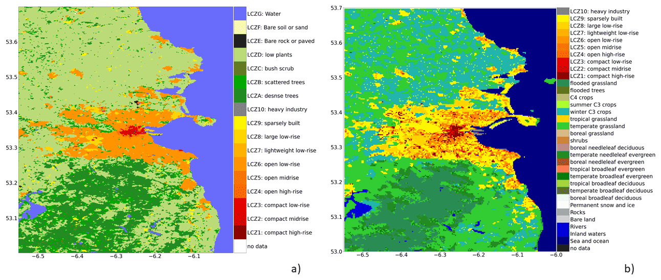
Figure 1Dublin area land cover map: (a) European Local Climate Zone (ELCZ2019) map (Demuzere et al., 2019), (b) ECOCLIMAP-Second Generation (ECO-SG) (CNRM, 2018).
This work is a continuation of the effort made by Met Éireann, the Irish Meteorological Service, to improve ECOCLIMAP (Masson et al., 2003; Faroux et al., 2013; CNRM, 2018), the default surface land-cover map used in cycle 43 of the HARMONIE-AROME canonical model configuration (CMC) of the shared ALADIN-HIRLAM NWP system for short-range operational weather forecasting (Bengtsson et al., 2017) used operationally at Met Éireann. The consortium for small scale modelling (COSMO) also has plans to use ECOCLIMAP for urban modelling (COSMO, 2022). The work started with an assessment of the latest version of ECOCLIMAP, ECOCLIMAP-Second Generation (ECO-SG hereafter) over Ireland. This assessment suggested that ECO-SG underestimates sparse urban areas which appear as vegetation – mostly grassland (Bessardon and Gleeson, 2019; Walsh et al., 2021). To correct ECO-SG issues, Sentinel-2 satellite images were segmented into various land-cover classes using a Convolutional Neural Network (CNN) following the Ulmas and Liiv (2020) method (Walsh et al., 2021). The resulting map, called the Ulmas–Walsh (UW) map, outperformed ECO-SG in terms of accuracy and resolution (Walsh et al., 2021). These encouraging results motivated efforts to implement the UW improvements in HARMONIE-AROME. However, before the UW map can be incorporated in HARMONIE-AROME, further work is needed on urban and vegetation land cover classes, the former of which is the focus of this paper.
The UW map uses the Coordination of Information on the Environment (CORINE) land cover database labels which differ quite significantly from the ECO-SG labelling system. There are 44 CORINE (tertiary) labels and 33 ECO-SG labels. CORINE includes mixed vegetation classes while ECO-SG uses pure vegetation types. Urban labels in CORINE reflect the function of the urban area (e.g. port, airport, roads) and the density of the urban area (discontinuous or continuous urban areas). In contrast, the ECO-SG urban labels consist of local climate zones (LCZ) (Stewart and Oke, 2012; CNRM, 2018).
Stewart and Oke (2012) introduced LCZs with the aim of standardising urban heat island studies. Urban climate-relevant parameters, such as imperviousness, sky view factor (SVF), the height of roughness elements, building surface fraction (BSF) or canyon aspect ratio (AR), define urban LCZ labels. This classification is extensively used by the urban climate community (Alcoforado et al., 2014; Alexander and Mills, 2014; Cai et al., 2018; Zheng et al., 2018) and led to the World Urban Database and Access Portal Tools (WUDAPT) method. This method relies on a supervised classification of urban areas using Landsat 8 imagery and Google Earth, and resulted in the production of the European local climate zone (called hereafter ELCZ2019) map (Demuzere et al., 2019).
Figure 1 compares the ELCZ2019 map over the Dublin area in Ireland against the same area using the ECO-SG classification. According to ECO-SG documentation (CNRM, 2018), the ECO-SG LCZ labels are defined using a combination of CORINE 2012 (Jaffrain, 2017) and the global human settlement layer maps (European Commission, 2022). Figure 1 shows that the ECO-SG LCZ labels for Dublin tend to be mostly LCZ9 (i.e. sparsely built areas – yellow) while the ELCZ2019 map shows a majority of LCZ6 (open low-rise – orange). ECO-SG also tends to represent vegetated areas, such as the Phoenix park (next to Dublin city centre), and the Howth peninsula (in the eastern part of the area) as LCZ9 (yellow) while in the ELCZ2019 map these areas are dominated by vegetation (greens). As shown in Walsh et al. (2021) CORINE classifies the Phoenix Park as an “Urban Green area”, which is translated as LCZ9 in ECO-SG (CNRM, 2018). While the Phoenix Park is by definition an “Urban Green area”, the translation to LCZ9 is questionable and reveals a need to validate and/or correct the ECO-SG LCZ classes.
The WUDAPT method is a reference method in the urban climate community, and as such, using the ELCZ2019 map, resulting from the WUDAPT method, could be an easy fix for ECO-SG urban deficiencies. However, Oliveira et al. (2020) list several studies that show limitations in the WUDAPT method and provide an alternative method for 5 Mediterranean cities using the CORINE dataset and Copernicus databases. This method proved to be highly accurate with an estimated 81 % overall accuracy and 90 % accuracy over urban LCZ (1–10) labels at 50 m resolution compared to 80 % overall accuracy at 100 m for ELCZ2019 (Demuzere et al., 2019).
One of the datasets used in Oliveira et al. (2020) is the Building Height 2012 dataset (European Environment Agency, 2018) which, regarding Ireland, is only available for Dublin (Sect. 2.3). There are no freely available building height data covering the entire island of Ireland. Recently, Frantz et al. (2021) combined Sentinel-1A/B and Sentinel-2A/B time series to map building heights for Germany. The training of this method used national building height information. In the study presented here, we used the Building Height 2012 dataset to apply the Frantz et al. (2021) method and compare it against other machine learning methods to obtain a building height map for the island of Ireland. The resulting building height map will help to classify the urban areas in the UW map as LCZ classes using Oliveira et al. (2020)'s method. This is needed in order for the UW map to become a direct replacement for ECO-SG over the island of Ireland in HARMONIE-AROME.
The paper is arranged as follows. Section 2 gives details about the Sentinel-1, Sentinel-2, Urban Atlas Building Heights, and the Settlement data used in this study. Section 3 provides details on the feature creation – the spectral indices and spectral and temporal features. Section 4 presents details of our approach to modelling while Sect. 5 presents the results of each model. Conclusions are provided in Sect. 6.
This section includes descriptions of the Sentinel-1 and Sentinel-2 satellite data used (Sect. 2.1 and 2.2), the building height information (Sect. 2.3) and the settlement data (Sect. 2.4).
2.1 Sentinel-1
The Sentinel-1 synthetic aperture radar (SAR) backscatter data for 2020 was retrieved from the Copernicus Open Access Hub API (Torres et al., 2012). For this study only ground range detected (GRD), high-resolution interferometric wide swath (IW) scenes were downloaded. These scenes contain backscatter intensities at 10 m pixel resolution for both the vertical transmit and vertical receive (VV) and vertical transmit and horizontal receive (VH) polarizations. In total ∼1057 ascending orbit scenes and ∼1325 descending orbit scenes cover the entire study area. As suggested by Koppel et al. (2017) Sentinel-1 data from both orbit directions were combined to enlarge the observation space. However, we found that this combination did not have a significant impact on model performance. In fact we found that just using the ascending orbit scenes provided an approximately equivalent performance with the added benefit of halving the pre-processing and download times (not shown). A workflow by Filipponi (2019) was applied to pre-process the Sentinel-1 (GRD) images to level 2 analysis-ready data using the SNAPPY module (more information can be found in Appendix E). Finally, the pre-processed Sentinel-1 images were re-projected onto the ”TM65/Irish Grid” projection and split into 30×30 km data cubes to match the sentinel-2 data (Frantz, 2019; Lewis et al., 2016).
2.2 Sentinel-2
The Google cloud platform was used to download the Sentinel-2 Level 1C scenes for the year 2020 which had a cloud coverage of less than 70 % (Google et al., 2022). Our entire study area is covered by 15 tiles (Military Grid Reference System see Fig. 2), which equates to 1310 (654 GB) Sentinel-2 scenes (containing both the S2A and S2B constellations). In order to produce Level 2 Analysis Ready Data (ARD), these raw Sentinel-2 scenes were processed through cloud and cloud shadow detection and radiometric calibration using the FORCE framework (Frantz, 2019) (more details can be found in Appendix F). All of the processed scenes were then re-projected to the same coordinate system as the Sentinel-1 scenes, and split into 30×30 km data cubes (Frantz, 2019; Lewis et al., 2016).
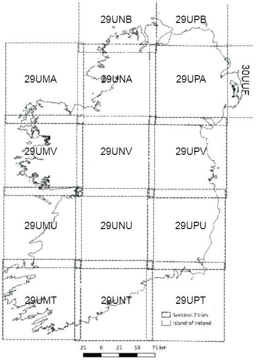
Figure 2This figure shows the 15 Sentinel 2 tiles needed to cover the entire Island of Ireland. The tile name is also included at the centre of each tile.
2.3 Building heights
The training and validation of any machine learning model requires ground truth labels. In our case accurate building height information was needed. For this study the data was gathered from the urban atlas dataset (European Environment Agency, 2018). This dataset contains a 10 m resolution raster layer that holds pixel-wise building height information for each capital city in Europe. The building height information is predicated on stereo images from the IRS-P5 Earth-imaging satellite and derived datasets such as the digital surface model (DSM), the digital terrain model (DTM) and the normalized DSM.
One drawback of this dataset is that it only covers Dublin city centre for the year 2012 and, unfortunately, does not have the resolution or correct metadata to discriminate between buildings and other man-made vertical structures. However, despite these limitations we used this dataset for modelling as it was the only freely available dataset at our disposal. Also for our application any vertical structure, regardless of its utility, will have an effect on LCZs. For modelling, this dataset was re-projected to the “TM65/Irish Grid” and converted to 30×30 km data cubes (Frantz, 2019).
2.4 Settlement data
Just as in Frantz et al. (2021), we used the European Settlement map (ESM) to mask the final predictions to areas covered by residential and non-residential buildings. The dataset was created using SPOT5 and SPOT6 satellite imagery and indicates the locations of human settlements throughout Europe (Copernicus, 2015). The settlement data was also re-projected to the “TM65/Irish Grid” and converted to 30×30 km data cubes using the FORCE software. The most recent version of this dataset is the 2015 version. Therefore, we updated the 2012 urban atlas building height dataset using the settlement map by masking out any buildings that were present in the urban atlas building height dataset but not in the more recent settlement map. Thus, the updated version is still not ideal, as we make the assumption that any buildings erected between 2012 and 2015 or even between 2012 and 2020 will not have significant impact on the model performance. The map is therefore limited to containing buildings that were present in both 2015 and 2012. Thus, the updated urban atlas building height dataset resembles the 2020 satellite images more closely, which in turn helps to produce a more accurate training dataset for the 4 models.
This section describes the steps applied to the satellite data to create features. A “Feature” refers to information gained from the satellite imagery that can be spectral, temporal and spatial in nature and feeds into the machine learning algorithms to predict building heights. Following the method of Frantz et al. (2021) we extracted a list of 1638 features from both the Sentinel-1 and Sentinel-2 time series data. Figure 3 presents an overview of the steps from the preparation of Sentinel-1 and Sentinel-2 data to the FORCE software, the creation of spectral indices, temporal features and spatial features. All of the feature engineering steps detailed in the following subsections were applied to the data using the FORCE framework (Frantz, 2020) on a t2.xlarge ubuntu instance on the Amazon Web Services (AWS) cloud platform, details of which can be found in the infrastructure subsection of Appendix A.
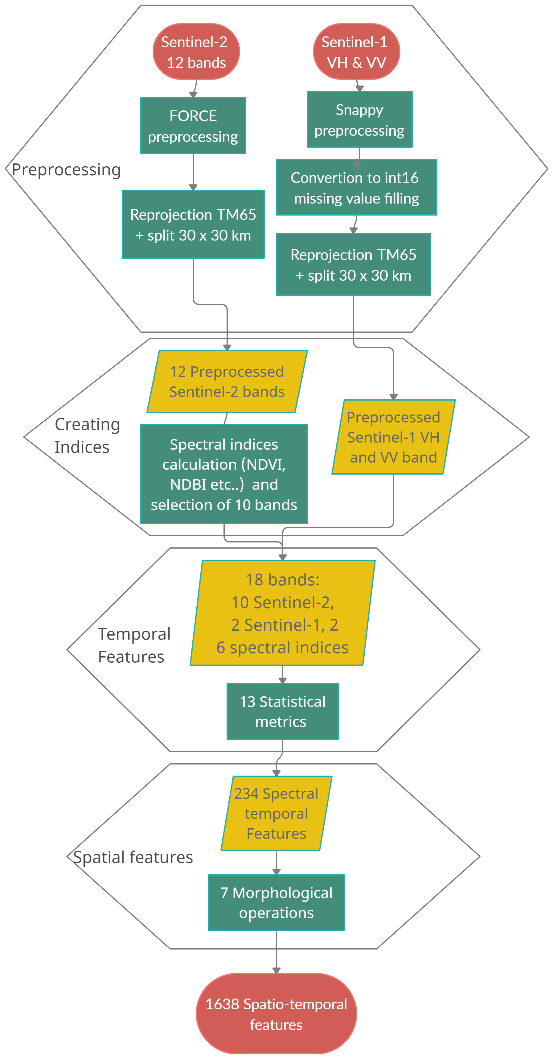
Figure 3A schematic of the data pre-processing workflow used for both the dataset creation and for producing the final building height map.
3.1 Spectral indices
The combination of Sentinel-1 and -2 data sources consists of 12 spectral bands, 2 of which are the VH and VV polarisations from the Sentinel-1 data with the rest coming from Sentinel-2 data. Just as in Frantz et al. (2021), in order to increase our model's accuracy we added 6 spectral indices derived from the optical Sentinel-2 bands. These indices include the Normalized Difference Vegetation Index (NDVI) (Tucker, 1979), Tasseled Cap Greenness (TCG) (Crist, 1985), Tasseled Cap Brightness (TCB) (Crist, 1985), Tasseled Cap Wetness (TCW) (Crist, 1985), Normalized Difference Water Index (NDWI) (Xu, 2006) and the Normalized Difference Built-Up Index (NDBI) (Zha et al., 2003). Both NDVI and TCG were chosen to improve the model's accuracy in detecting urban vegetation which was a problem area in the Li et al. (2020) Sentinel-1-only study. NDBI was also included for its capability in detecting urban areas. TCW and NDWI were chosen because they can potentially detect moisture on the surfaces of urban areas, which can distort shadow lengths. The final index included was TCB which captures the difference in reflectance from different roofing materials and shapes. All of these indices are provided as part of the higher level processing functions supplied by the FORCE framework (see FORCE in Appendix C). In total we therefore had 18 bands/indices to work with.
3.2 Temporal features
There are seasonal features in the Sentinel time series data that are affected directly by building heights, such as reflectance and shadow lengths caused by changes in the Sun's path (Frantz et al., 2021). In order to capture these seasonal effects we created pixel-wise statistical aggregations for all of the quality pixel values for the entire time period (2020). As we have the same scene over time (on average each scene will be captured 40–60 times throughout the year), each pixel or (X, Y) point in the scene will have a distribution of values that span the entire time period. This distribution of pixel values is used to calculate statistical metrics. Due to their robustness against missing data and spatial completeness these metrics are incredibly useful for machine learning applications (Rufin et al., 2019; Schug et al., 2020).
Because the quality of the Sentinel-2 optical scenes is dependant on weather conditions, only clear-sky, non-cloud, non-cloud shadow and non-snow pixels were considered. Whereas for the Sentinel-1 radar data all observations can be used. We applied all of the 13 statistical metrics available in FORCE (Frantz, 2019) to each of the 18 bands/indices (2 from Sentinel-1, 10 from Sentinel-2 and the 6 new spectral indices). The metrics included: average, standard deviation, 0 %/10 %/25 %/50 %/75 %/90 %/100 % quantiles, the interquartile range, kurtosis and skewness. For example, if you consider the top left pixel in a scene, this pixel will have 40–60 different values as the scene has been captured multiple times throughout the year. This means for every (X, Y) point in a scene we have a distribution of pixels over time. This is the distribution that is used to create our statistical aggregations. For example, the maximum aggregation is the maximum value in this distribution. This is done for each (X, Y) point in the scene and for each band which results in 234 spectral temporal features, as we applied all 13 statistical metrics to each of the 18 bands/indices.
3.3 Spatial features
To capture the spatial context of the surrounding pixels we applied 7 different morphological operators across the 234 spectral temporal features previously created. These operators included Dilation, Erosion, Opening, Closing, Gradient, Tophat and Blackhat. Morphology is a standard image processing technique where a structuring element is applied across the entire scene to capture spatial context. The structuring element works by turning on or off certain pixels depending on their position in the structuring element which in turn captures different spatial aspects of the surrounding pixels. Just as in Frantz et al. (2021), 7 morphological operations were used, all of which utilised a circular structuring element with a 50 m radius or 5 pixels at 10 m resolution. Again this process was executed through the texture features supported by the FORCE framework (Frantz, 2019). This step was applied to each of the 234 features. Thus, the final dataset for modelling contained 1638 features.
This section details our approach to modelling, including sampling the reference building height data in order to train, validate and select the most relevant features for our models; the feature selection method; and a presentation of the models along with the metrics used to evaluate their performance.
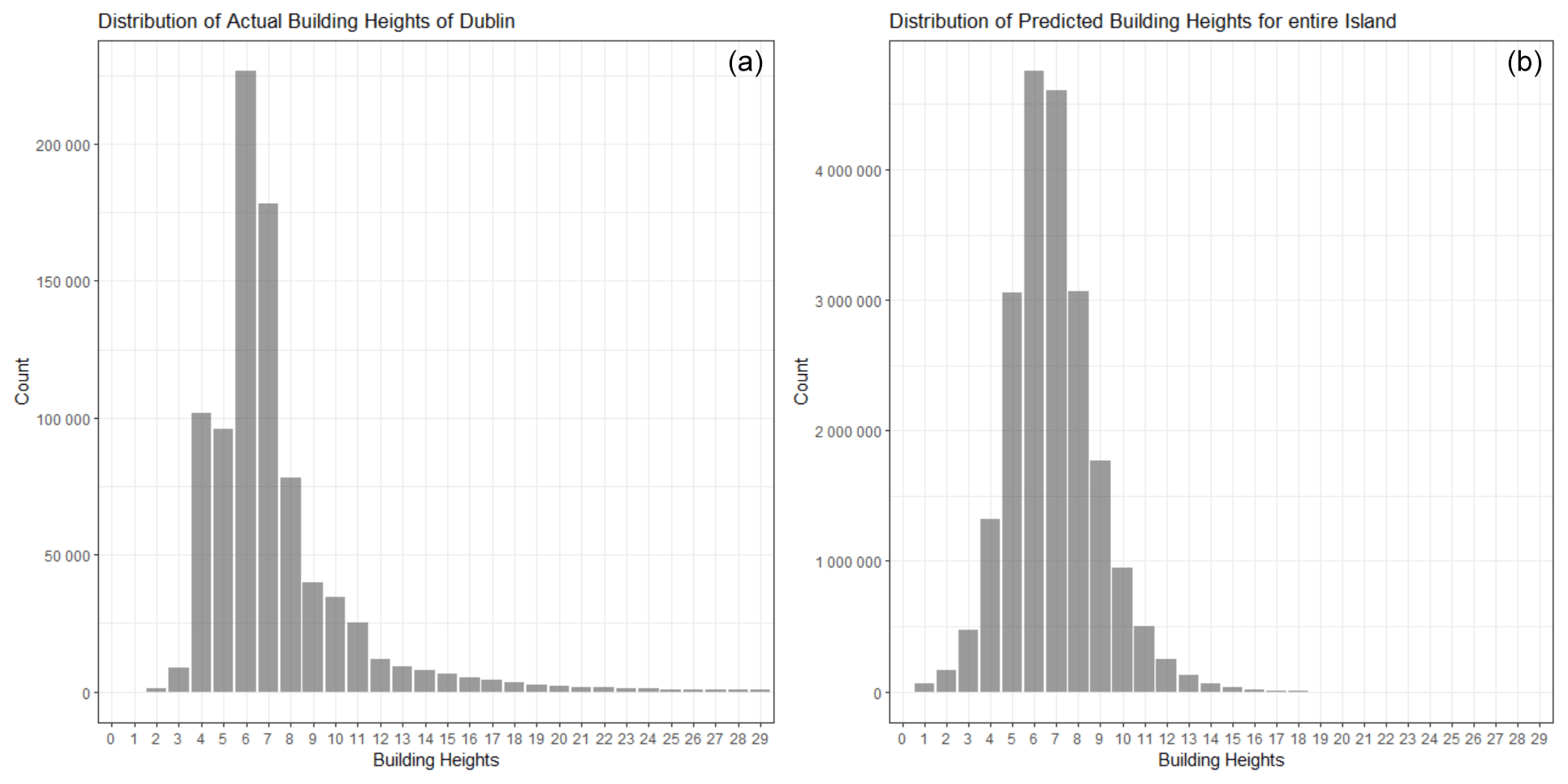
Figure 4Building height distribution from the Urban Atlas 2012 for Dublin City (a), final building height predictions for the entire island of Ireland (+20 million pixels) using the Ridge Regression model (b). Only Buildings in the [0; 29] m range were included for visualisation purposes. (a) has a mean value of 7.28 m and a standard deviation of 3.61 m. Whereas (b) has a mean value of 6.53 m and a standard deviation of 2.02 m
4.1 Sampling for training and validation
As with any typical machine learning workflow, we created a training dataset which comprised of 1 048 576 samples and a hold-out dataset of 264 596 samples, both of which included all of the 1638 features described in Sect. 3. The training dataset was used to train each of the models. Whereas, the hold-out dataset was used to fairly measure their performance, as the models have not been exposed to these samples beforehand. For fairness of evaluation both the training and hold-out datasets were created using a stratified sampling approach. This approach maintains the same building height distributions for both the training and hold-out datasets and creates a more realistic indication of model performance. The distribution of the known buildings heights of Ireland in the urban atlas (see Fig. 4) was used to create these stratified samples. Areas with no buildings were also added to the dataset with a height value of zero. This was accomplished by selecting a random point on the image and checking whether any non-zero building heights are within a 100 m radius. If no buildings exist then the sample was added to the dataset otherwise it was skipped. This process was repeated until 4.9 % of the total number of samples were filled. This value was chosen as it is the average value when the building height distribution is converted from counts to percentages.
4.2 Feature selection
With 1638 features in total the feature-space is too large and, due to the “curse of dimensionality” this can lead to over-fitting and unnecessary computational complexity when constructing the building height map. By using a feature selection tool we can reduce over-fitting by removing noisy features. This increases the model's ability to generalise to unseen data and increases accuracy. We performed the feature selection step on our training dataset using the BorutaShap algorithm (Keany, 2020). This algorithm selected 64 features that performed better than random noise in predicting building heights, 37 of which were based on Sentinel-2 data with the rest derived from Sentinel-1 data. From Fig. 5 we can see that 13 of the 18 bands/indices were found to be important in predicting building heights. The vertical and horizontal bands/indices from Sentinel-1 were found to be the most import features for predicting building heights, closely followed by the NIR, NDWI and TCG bands/indices. Similarly, 5 out of 7 morphological operations and 11 of the 13 statistical aggregations were useful. The Dilation and Erosion morphological operators and the 50 % quartile, minimum and 10 % quantile were found to be the most important morphological operations and statistical aggregations respectively, see Sect. 3 for the origin of these features.

Figure 5The top left figure describes the 10 most important features when predicting building heights. The remaining three figures show the importance of the different features from each of the previous feature engineering steps in Sect. 3. These three plots were created by aggregating the importance (measured in shapely values; Lundberg and Lee, 2017) of all of the 64 features that included these feature steps, either band, morphology or STM. The feature names in the top left chart are a combination of features from the other 3 graphs, example “NDW Q50 DIL” → the 50th quartile of the Normalized Difference Water Index.
4.3 Models presentation
In order to expand the work of Frantz et al. (2021), we compared the performance of 4 models. In essence we have two distinct categories of model, tabular and Convolutional Neural Network (CNN) architectures. Tabular models expect the data in the form of a table (see Fig. 6) where each row is a pixel and the columns are the 64 selected features, whereas CNN architectures leverage the spatial context of the scenes themselves.

Figure 6A schematic illustrating how the satellite images were converted into a table format necessary for model consumption. The image volume on the left contains the 1638 features created for a single scene or area of interest. Each pixel in the image stack is converted into a row in the table. We store the X and Y location of the pixel in the image and the 1638 features are converted to columns.
The two tabular models used were a Ridge Regressor (Van Wieringen, 2018) and a Poisson XGBoost Regressor (Chen and Guestrin, 2016). The Ridge Regressor was the only linear model used, and provided us with a baseline performance. This model was chosen for its L2 regularisation which combats over-fitting by reducing the model's bias and variance, especially in our case where the independent variables are highly correlated. To improve upon the baseline accuracy of this linear model we trained a state-of-the-art XGBoost Regressor. This model uses gradient boosted decision trees that allow it to capture non-linear trends in the data which in theory will improve the model’s accuracy scores. The Poisson objective function was heuristically chosen, from a visual inspection of our building height distribution (which only contains integer values). During modelling, this objective function provided the best performance for our XGBoost Regressor (not shown).
Steering away from tabular models, two CNN architectures were applied to our data as they have an inherent capacity to handle internal spatial context. A CNN is a sub-class of neural networks containing multiple convolution layers. These layers are great for automatically capturing local spatial information, as well as reducing the overall complexity of the model. Unlike tabular models, CNNs do not need the images to be transformed to a tabular data structure. They can simply ingest the entire image at once. While most CNN architectures only use 3 features (RGB) we adjusted our CNN models to be able to use the top 5 features selected in Sect. 4.2. Five input features were chosen as they allow the CNN architecture to capture the spatial context on its own while reducing the overall complexity of the model relative to choosing a larger number of input channels (not shown).
The two CNN architectures used were a simple CNN inspired by LeCun et al. (1999) and an U-Net (Ronneberger et al., 2015) style encoder decoder CNN architecture. The architecture inspired by LeCun et al. (1999) has 7 layers including 2 convolutional layers with 3455×5 kernels, 2 average pooling layers, and an input, hidden and output layer. Rectified Linear Units (ReLUs) were also used for activation in all layers. The computational complexity required to make predictions on a large scale can be an obstacle in using this model.
In an attempt to reduce this computational complexity a convolutional encoder decoder style network was fitted to the training data, as we believed that this style of model should have both the speed and accuracy needed. The model was based on the U-Net (Ronneberger et al., 2015) architecture with two adjustments: the typical RGB input was replaced with our top 5 features and the loss metric was replaced with the weighted root mean square error (wRMSE) as U-Net is typically applied to image segmentation not pixel wise regression.
4.4 Model training and evaluation metrics
Both tabular models (Ridge Regressor and a Poisson XGBoost Regressor) were trained using the 64 most important features derived from the VV/VH Sentinel-1A/Band multi-spectral Sentinel-2A/B time series data selected in (section 4.2). The model hyper-parameters were tuned using a random search combined with a 10-fold cross-validation, and all pixels with a building height value of zero were removed. For the Ridge Regressor, the target distribution was transformed into a normal distribution using a Yeo–Johnson transformation, while for the XGBoost model we kept the original distribution and instead changed the model's objective function to a Poisson count distribution.
To train both of our CNN architectures, the same dataset was used but only the 5 most important spectral temporal features were included as shown in Fig. 5:
-
the 10th quantile of VV band;
-
the minimum of the VH band;
-
the 50th quartile of the NIR band;
-
the average of the TCB band;
-
the 50th quartile NDVI.
To evaluate each model's performance we applied 4 metrics to the predictions and the ground truth building heights provided by the Urban Atlas. The Root Mean Square Error (RMSE) was the base metric for assessing model performance. However, the RMSE value is slightly skewed towards taller buildings. These taller buildings (above 15 m) are a rare occurrence within the building height distribution especially outside of the major cities. Therefore, to create a more realistic metric a wRMSE metric was used where the RMSE error for each building was weighted by the frequency of height occurrences. This provides a more realistic metric especially as we extrapolated the model over the entire island of Ireland where tall buildings are practically non-existent outside of major cities.
We further compared the predicted building height distributions produced by each of the models. For each model we compared the normalised histograms of their building height predictions against the actual building heights (from the Urban Atlas) by computing the Earth Mover's distance metric (EOD) on the hold out dataset. The EOD represents the distance between two probability distributions and thus gives a numerical representation to accompany the visual inspection of the histograms. This approach was adopted to ensure that the chosen model could produce a realistic and varied building height distribution instead of producing an accurate distribution centred around the mean. Finally, we also measured the time taken for each model to make its predictions for one 100 km × 100 km tile from the Military Grid Reference System (see Fig. 2). This metric was important as we needed to strike a balance between accuracy and computational complexity for our prospective model.
The performance of each model with respect to our predefined metrics is captured in Table 1. The CNN consistently outperforms the other models achieving the best results for RMSE, wRMSE, and Earth Mover's distance. This superior performance is expected, as CNN architectures have been shown to consistently outperform classical computer vision methods. Despite this success, the CNN model has 10× the computational complexity of the tabular models, adding an extra 13 d of processing time to our map construction (with the same hardware). This excessive computational complexity is not caused by the model, but instead by the data extraction needed to make a prediction. In order to make a prediction we need to loop through the entire image pixel by pixel and then extract the surrounding pixels for each pixel of interest. For tabular models the image can first be converted into a table (see Fig. 6) with each row representing a building height and the columns the 64 features determined in the feature selection process. This table can be easily masked by the settlement map and the predictions transformed back into a raster image format.
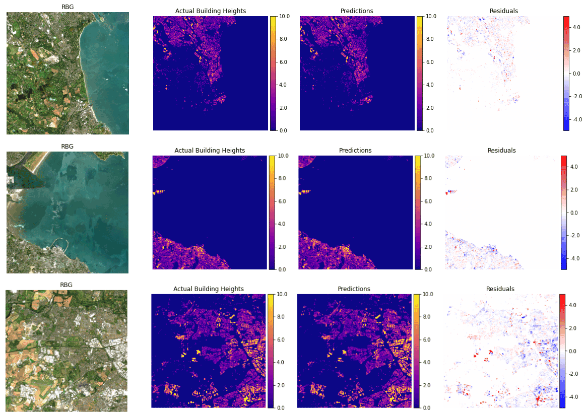
Figure 7This Figure displays three 10 km × 10 km sample predictions from the Ridge Regression model. From left to right: the first image is an RGB representation of the scene using data provided by the Sentinel-2 satellite (Drusch et al., 2012), next is the actual building heights for the scene, then the model prediction and the last image is the residuals of the predictions.
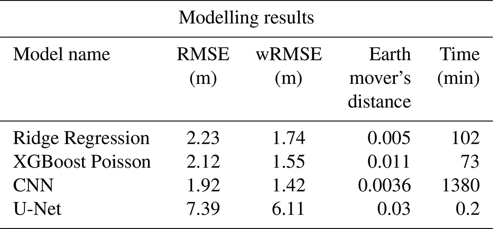
Table 1The Performance of each model with respect to the 4 metrics (RMSE, WRMSE, EOD and Time to create a single Military Grid Tile) defined in Sect. 4.4.
The CNN encoder decoder based on the U-net architecture was expected to have both speed and accuracy. However, when tested on the hold-out dataset this model performed poorly with a RMSE of 7.39 m and a wRMSE of 6.11 m. After a visual inspection of the predicted height distribution, we noticed that the model was producing a trivial solution where every prediction was closely centred around the mean value (see Fig. 10). Despite this, we tried numerous different approaches including reducing the training image sizes to 1.28 km × 1.28 km, 640 m × 640 m and 280 m × 280 m, creating a new loss function similar to Eigen and Fergus (2015), adding image augmentations and using only the RGB bands with a pre-trained ResNet model as the Encoder block (He et al., 2016). Unfortunately, none of these changes had a positive effect on the model's accuracy in terms of wRmse, RMSE, EOD. The literature is quite sparse for building height estimation with convolutional encoder decoder networks. The only work found used a pre-trained ResNet model on RGB bands, without the temporal aspect, and at 2 m resolution (Mou and Zhu, 2018). However, during the feature selection process we learned that at 10 m resolution, with a temporal aspect, the red and blue bands performed worse than random at predicting building heights. Thus, we speculate that the under-performance of the U-Net model could be attributed to the lack of high resolution data (10 m vs. 2 m) and the small number of training images, approximately 300 images excluding augmentations.
The XGBoost model achieved the second lowest time to create a single tile, only second to the convolutional encoder decoder network. This is not a surprise as this model was designed for speed and performance (Chen and Guestrin, 2016). During hyper-parameter tuning it was discovered that using the Poisson objective out-performed the default squared error objective function in all of our accuracy aspects (not shown). This Poisson XGBoost model out-performed our Ridge Regression model in both RMSE and wRMSE. However, on visual inspection it produced a more unrealistic height distribution as shown in Fig. 10. This fact is echoed by the relatively large EOD (Table 1). The model clearly under-predicts heights at the tails of the distribution while grossly over-predicting the average building height (7 m).
In terms of accuracy, the Ridge Regressor model had the highest RMSE and wRMSE scores of the 3 models (CNN, XGBoost, Ridge Regressor) that produced a reasonably realistic output. This suggests that there must be some non-linear interactions that cannot be captured relative to the other two non-linear models. We can see from Fig. 10 that the Ridge Regressor model under-predicts the tails of the distribution but overall it produces a much more realistic height distribution compared to the XGBoost model. This realistic distribution and the model's computational complexity relative to the CNN made the Ridge Regressor the optimal choice for producing the national scale map. Despite having the largest RMSE and wRMSE values of the 3 models that produced a realistic output, the discrepancy between the RMSEs and wRMSEs is less than 30 cm. This accuracy discrepancy will not have a serious impact on creating maps in future studies such as for the LCZs, as we only need to categorize the heights into high-rise, mid-rise and low-rise areas. With our chosen model we recreated three 10×10 km areas from our hold-out dataset (which can be seen in Fig. 7). Despite training our models using a pixel-wise representation of building heights, this method is clearly capable of producing a realistic output. The maximum residual error of any pixel in the 3 segments is ±5 m. However, in certain areas the residuals can be seen to fluctuate from pixel to pixel. In the future this problem could be solved using a post processing technique to smooth out the sudden changes to create a more locally consistent map.
Our final ridge Ridge Regressor was trained on 100 % of the available data. The resultant building height map can be seen in Fig. 8 and a more granular view of the 4 major cities in Ireland can be seen in Fig. 9. The distribution of the building height predictions in the final map can be seen in Fig. 4. The graph on the left represents the total distribution of building heights for Dublin City in 2012 (these were the heights used to train the models). This distribution has a mean of 7.28 m and a standard deviation of 3.61 m. The graph on the right shows the distribution of predicted building heights for the island of Ireland by our final Ridge Regression Model. This distribution has a mean of 6.53 m and a standard deviation of 2.02 m. The predicted building height distribution is normally distributed and is limited to the range 0–21 m. In reality, we expect the building height distribution for the entire country to be right skewed as smaller buildings are much more prevalent then taller buildings. If a more varied training dataset, that represented Ireland as a whole rather than just Dublin city, was available then the resultant building height distribution may align more with our expectations. Despite this, it is evident from Fig. 7 that our final Ridge Regression Model clearly produces a realistic output; the first image has an RMSE of 1.32 m, wRMSE of 1.77 m and an Earth Mover's Distance (EOD) of 0.0022. The second has an RMSE of 2.29 m, wRMSE of 1.56 m and an EOD of 0.0036. The final image has an RMSE of 2.0 m, wRMSE of 1.62 m and an EOD of 0.0029.

Figure 8The final building height map created from our models predictions. The colour scale has been limited to 0–15 m for visualisation purposes.
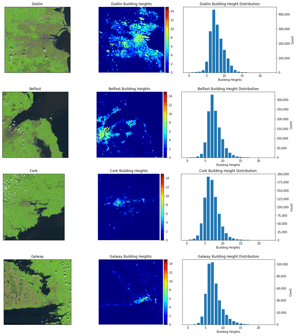
Figure 9The final model predictions for the 4 main cities of Ireland Dublin, Belfast, Cork and Galway. From left to right the images are the RGB satellite view of the given city using data provided by the Sentinel-2 satellite (Drusch et al., 2012). The building heights predicted by our final model and the right hand graph shows the distribution of the predicted building heights. The colour scale in the middle graphs has been limited to 0–15 m for visualisation purposes.
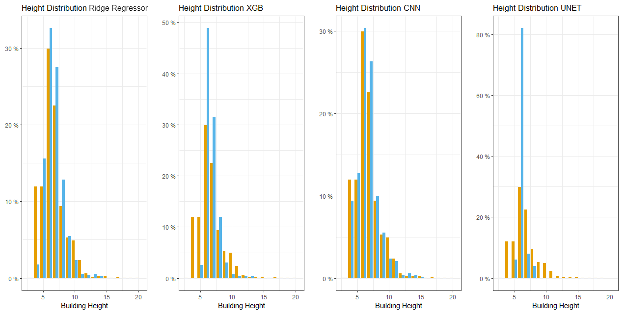
Figure 10Orange bars represent building heights and the blue bars represent the predicted building heights for each model. From left to right the four graphs represent the Ridge Regressor, XGBoost Regressor, CNN and U-Net models.
In summary, this paper demonstrates a workflow to produce a cost-effective building height map at a national scale. The proposed methodology relies completely on freely available data, open source software and the AWS cloud platform. This accessibility allows any country within the European Union to produce their own map either using the AWS platform or their own computer resources. A thorough feature selection process was carried out, that deemed 64 spectral-temporal-spatial features to be important when predicting building heights at a 10 m resolution. Using these features the prediction quality, accuracy and computational complexity of several models was explored. Despite having relatively large RMSE (2.23 m) and wRMSE (1.74 m) values, the Ridge Regression model provided the optimal blend of a low computational overhead paired with a realistic output. Depending on the application and access to computational resources, the more accurate, but computationally expensive, CNN could be used.
This approach is not perfect, and is limited to producing a 10 m resolution map. Therefore, the actual heights of specific buildings are not attainable which may not suit certain applications. The resultant map is also constrained by the Copernicus open source datasets. This caused a discrepancy between the training dataset for the 4 models because the satellite imagery was from 2020 but our building heights were from 2012. The resultant map was also constrained to the year the settlement map was produced (2015). However, as all of the data needed to create the building height map are open source, the described workflow can be re-implemented once new updated versions of these data sources become available. This has the added benefit of not only updating our map but producing a more accurate map, once all of the data sources become available for the same year.
In the future, the resulting complete building height map will be combined with urban density data to correctly classify urban LCZs. These urban LCZs will be used to update the existing land cover map in HARMONIE-AROME over Ireland. In conclusion, this methodology produces a cost effective building height map that could have numerous different applications outside of numerical weather prediction. This could benefit any EU Member State, covered by the Copernicus datasets, which have no access to open access countrywide building height data.
We used the AWS cloud platform to provide the necessary computing power for this project. If you have access to appropriate computer and storage resources then this section can be skipped. In order to process a single tile we need two ec2 cloud instances/servers – the first to process the Sentinel-1 data and the other the Sentinel-2 data. Both were t2.xlarge instances which have the following specifications: 4 virtual CPUs and 16 GB of RAM. The size of the instance was chosen as this is the minimum specification needed to successfully run the FORCE software. Both instances ran UBUNTU 18.04 and the FORCE software. The Sentinel-1 instance also required ESA SNAP software and the SNAPPY python package to run the Sentinel-1 processing pipeline. Both of these instances were attached to a shared 600 GB EBS volume to store the associated data. This setup allowed us to comfortably process a single tile. In order to process multiple tiles in parallel we recreated this infrastructure setup 5 times with the help of the AWS console. This allowed us to create 5 tiles in parallel decreasing the overall time to create the map. This cloud infrastructure setup allowed us to create a 10 000 km2 section for only EUR 6.
As mentioned in the main part of the paper Ireland is covered by 15 tiles (Military Grid Reference System, see Fig. 2). For ease of construction we processed each tile separately. This had the added benefit of horizontal scaling, as multiple smaller machines can process tiles in parallel. Each tile took approximately 24 h to process. The deviation in processing time was caused by the content of each tile. Tiles that were located on the coast took less time on average as the ocean values are not processed by the FORCE software. Also the size of the area covered by built-up infrastructure affects the time taken to process a tile. On average each tile cost EUR ∼6 to produce. In total we were able to produce our entire map in 3 d at a total cost of EUR ∼80.
The FORCE framework is an all-in-one processing engine for medium-resolution Earth Observation image archives. FORCE allows the user to perform all of the essential tasks in a typical Earth Observation Analysis workflow, i.e. going from data to information. FORCE supports the integrated processing and analysis of:
-
Landsat TM;
-
Landsat 7 ETM+;
-
Landsat 8 OLI;
-
Sentinel-2 A/B MSI.
Non-native data sources can also be processed by FORCE, such as Sentinel-1 SAR data. In order to use the FORCE framework the Sentinel-1 data needs to be prepared in a FORCE-compatible format. The images need to be in the correct tiling scheme with signed 16 bit integers and scaled backscatter in the order of −1000 s. No data values need to be assigned as −9999. The data need to have two bands: VV and VH, and the image name should follow the standard FORCE naming structure: date, sensor and orbit e.g. 20180108_LEVEL2_S1AIA_SIG.tif (Frantz, 2019).
Developed by the European Space Agency (ESA), the Sentinel Application Platform (SNAP) is a common software platform that supports the Sentinel missions. The toolbox consists of several modules that can be used for image processing, modelling and visualisation. SNAP is not only a research support tool for the Sentinel missions (Sentinel-1, Sentinel-2 and Sentinel-3) but a functional tool that can be leveraged to process large amounts of satellite data (European Space Agency, 2021). In order, to use the SNAP toolbox through python, SNAPPY is required. SNAPPY is essentially a Python module that allows the user to interface with the SNAP API, through the Python programming language (Culler et al., 2021).
A workflow by Filipponi (2019) was applied to pre-process the Sentinel-1 (GRD) images to level 2 analysis-ready data. Level 2 analysis ready refers to the quality of the satellite scenes (European Space Agency, 2015). To accomplish this a pre-processing pipeline was created using a python interface (SNAPPY) for the SNAP sentinel-1 toolbox (Culler et al., 2021) and the freely available 3 arcsecond Shuttle Radar Topography Mission (SRTM) terrain model (Farr et al., 2007). The first processing step was to apply the precise orbit files available from SNAP to the Sentinel-1 products, in order to provide accurate satellite position and velocity information. Border noise effects, which affect a percentage of the original Sentinel-1 scenes, were also eliminated along with thermal noise. The SRTM terrain model was then used to apply Range Doppler terrain Correction to correct for distortions in the scene caused by the varying viewing angle greater than 0∘ of our sensor. This varying angle causes some distortion related to side-looking geometry. Range Doppler terrain corrections are intended to compensate for these distortions so that the geometric representation of the image will be as close as possible to the real world (Filipponi, 2019). The final step in the workflow was to convert the processed backscatter images to the decibel scale. In order to use the higher level processes from the Framework for Operational Radiometric Correction for Environmental monitoring (FORCE) (Frantz, 2019) all of these processed Sentinel-1 scenes had to be converted to a compatible format.
The raw Sentinel-2 scenes were processed to Level 2 Analysis Ready Data (ARD) through the FORCE framework by Frantz (2019) available at Frantz (2020). This open source framework conducts all of the necessary steps involved to produce level 2 (ARD) products. These processes include cloud and cloud shadow detection using a modified version of the Fmask algorithm (Frantz et al., 2016) and radiometric calibration which also uses the freely available 3 arcsec SRTM terrain model (Farr et al., 2007). A more in-depth description of all of the processes applied during the level 2 ARD workflow can be found in Frantz (2019).
The code used for this project can be found at https://doi.org/10.5281/zenodo.6501910 (Keany, 2022). The data used to obtain the results are open-source and available at the following web addresses: Urban atlas 2012 dataset: https://land.copernicus.eu/local/urban-atlas/building-height-2012 (European Environment Agency, 2018) and https://ghsl.jrc.ec.europa.eu/ (European Commission, 2022), Sentinel-1 and Sentinel-2 Satellite Data: https://scihub.copernicus.eu/ (European Space Agency, 2022).
All three authors EG, GB and EK contributed to the writing of this paper. EK wrote the code and executed all of the experiments.
The contact author has declared that neither they nor their co-authors have any competing interests.
Publisher's note: Copernicus Publications remains neutral with regard to jurisdictional claims in published maps and institutional affiliations.
This article is part of the special issue “21st EMS Annual Meeting – virtual: European Conference for Applied Meteorology and Climatology 2021”.
The authors would like to acknowledge David Frantz and Stefan Ernst for creating and maintaining the FORCE framework and Jan-Peter Schulz and Polina Shvedko for reviewing the manuscript and providing useful suggestions.
This paper was edited by Daniel Reinert and reviewed by Jan-Peter Schulz and one anonymous referee.
Alcoforado, M. J., Lopes, A., Alves, E. D. L., and Canário, P.: Lisbon Heat Island, Finisterra, 49, 61–80, https://doi.org/10.18055/Finis6456, 2014. a
Alexander, P. J. and Mills, G.: Local climate classification and Dublin's urban heat island, Atmosphere, 5, 755–774, https://doi.org/10.3390/atmos5040755, 2014. a
Bengtsson, L., Andrae, U., Aspelien, T., Batrak, Y., Calvo, J., de Rooy, W. C., Gleeson, E., Hansen-Sass, B., Homleid, M., Hortal, M., Ivarsson, K.-I., Lenderink, G., Niemelä, S., Nielsen, K. P., Onvlee, J., Rontu, L., Samuelsson, P., Muñoz, D. S., Subias, Á., Tijm, S., Toll, V., Yang, X., and Køltzow, M.: The HARMONIE-AROME Model Configuration in the ALADIN-HIRLAM NWP System, Mon. Weather Rev., 145, 1919–1935, 2017. a
Bessardon, G. and Gleeson, E.: Using the best available physiography to improve weather forecasts for Ireland, in: Challenges in High Resolution Short Range NWP at European level including forecaster-developer cooperation, European Meteorological Society, Lyngby, https://presentations.copernicus.org/EMS2019/EMS2019-702_presentation.pdf (last access: 28 March 2022), 2019. a
Cai, M., Ren, C., Xu, Y., Lau, K. K. L., and Wang, R.: Investigating the relationship between local climate zone and land surface temperature using an improved WUDAPT methodology – A case study of Yangtze River Delta, China, Urban Clim., 24, 485–502, https://doi.org/10.1016/J.UCLIM.2017.05.010, 2018. a
Chen, T. and Guestrin, C.: Xgboost: A scalable tree boosting system, in: Proceedings of the 22nd acm sigkdd international conference on knowledge discovery and data mining, 13–17 August 2016, San Francisco, California, USA, 785–794, https://doi.org/10.48550/arXiv.1603.02754, 2016. a, b
CNRM: Wiki – ECOCLIMAP-SG – CNRM Open Source Site, https://opensource.umr-cnrm.fr/projects/ecoclimap-sg/wiki (last access: 28 April 2022), 2018. a, b, c, d, e, f
Copernicus: Settlement map 2015, https://land.copernicus.eu/pan-european/GHSL/european-settlement-map (last access: 13-August-2021), 2015. a
COSMO: Priority Project CITTA, https://www.cosmo-model.org/content/tasks/priorityProjects/citta/default.htm (last access: 28 April 2022), 2022. a
Crist, E. P.: A TM tasseled cap equivalent transformation for reflectance factor data, Remote Sens. Environ., 17, 301–306, 1985. a, b, c
Culler, M., Dunfield, N. M., Goerner, M., and Weeks, J. R.: SnapPy, a computer program for studying the geometry and topology of 3-manifolds, http://snappy.computop.org (last access: 11 April 2022), 2021. a, b
Demuzere, M., Bechtel, B., Middel, A., and Mills, G.: Mapping Europe into local climate zones, PLoS ONE, 14, 1–2, https://doi.org/10.1371/journal.pone.0214474, 2019. a, b, c, d
Drusch, M., Del Bello, U., Carlier, S., Colin, O., Fernandez, V., Gascon, F., Hoersch, B., Isola, C., Laberinti, P., Martimort, P., Moon, S., Oldeman, P., Palomba, M., Patterson, J., Prochazka, M., Schricke-Didot, M. H., Schwieso, C., Skoog, J., Spoto, F., Stjernevi, J., Sy, O., Teianu, B., Wildner, C., Arino, O., Bargellini, P., Berger, M., Cadau, E. G., Ferran Gascon, O. C., Hoersch, B., Laur, H., López Fernández, B., Monjoux, E., Baker, M., Marchese, F., and Pineiro, J.: Sentinel-2: ESA's optical high-resolution mission for GMES operational services, Remote Sens. Environ., 120, 25–36, 2012. a, b
Eigen, D. and Fergus, R.: Predicting depth, surface normals and semantic labels with a common multi-scale convolutional architecture, in: Proceedings of the IEEE international conference on computer vision, 7–13 December 2015, Santiago, Chile, 2650–2658, https://doi.org/10.48550/arXiv.1411.4734, 2015. a
European Commission: GHSL – Global Human Settlement Layer, https://ghsl.jrc.ec.europa.eu/, last access: 28 April 2022. a, b
European Environment Agency: Copernicus Land Service – Pan-European Component: CORINE Land Cover, https://www.eea.europa.eu/data-and-maps (last access: 28 April 2022), 2017. a
European Environment Agency: Building Height 2012, European Environment Agency [data set], https://land.copernicus.eu/local/urban-atlas/building-height-2012 (last access: 28 April 2022), 2018. a, b, c
European Space Agency: Sentinel 2 User Handbook, https://sentinel.esa.int/documents/247904/685211/Sentinel-2_User_Handbook (last access: 13 August 2021), 2015. a
European Space Agency: Land Cover CCI Product User Guide Version 2.0, http://maps.elie.ucl.ac.be/CCI/viewer/download/ESACCI-LC-Ph2-PUGv2_2.0.pdf (last access: 28 April 2022), 2017. a
European Space Agency: Sentinel Application Platform (SNAP), https://step.esa.int/main/toolboxes/snap/ (last access: 28 April 2022), 2021. a
European Space Agency: Copernicus Open Access Hub, https://scihub.copernicus.eu/, last access: 28 April 2022. a
Faroux, S., Kaptué Tchuenté, A. T., Roujean, J.-L., Masson, V., Martin, E., and Le Moigne, P.: ECOCLIMAP-II/Europe: a twofold database of ecosystems and surface parameters at 1 km resolution based on satellite information for use in land surface, meteorological and climate models, Geosci. Model Dev., 6, 563–582, https://doi.org/10.5194/gmd-6-563-2013, 2013. a
Farr, T. G., Rosen, P. A., Caro, E., Crippen, R., Duren, R., Hensley, S., Kobrick, M., Paller, M., Rodriguez, E., Roth, L., Seal, D., Shaffer,S., Shimada, J., Umland, J., Werner, M., Oskin, M., Burbank, D., and Alsdorf, D.: The shuttle radar topography mission, Rev. Geophys., 120, 25–36, https://doi.org/10.1016/j.rse.2011.11.026, 2007. a, b
Filipponi, F.: Sentinel-1 GRD Preprocessing Workflow, Proceedings, 18, 19, https://doi.org/10.3390/ECRS-3-06201, 2019. a, b, c
Frantz, D.: FORCE – Landsat+ Sentinel-2 analysis ready data and beyond, Remote Sens., 11, 1124, https://doi.org/10.3390/rs11091124, 2019. a, b, c, d, e, f, g, h, i, j
Frantz, D.: FORCE Documentation, https://force-eo.readthedocs.io/en/latest/ (last access: 13 August 2021), 2020. a, b
Frantz, D., Röder, A., Stellmes, M., and Hill, J.: An operational radiometric landsat preprocessing framework for large-area time series applications, IEEE T. Geosci. Remote, 54, 3928–3943, 2016. a
Frantz, D., Schug, F., Okujeni, A., Navacchi, C., Wagner, W., van der Linden, S., and Hostert, P.: National-scale mapping of building height using Sentinel-1 and Sentinel-2 time series, Remote Sens. Environ., 252, 112128, https://doi.org/10.1016/j.rse.2020.112128, 2021. a, b, c, d, e, f, g, h
Google, European Space Agency, and Copernicus: Sentinel-2 MSI: MultiSpectral Instrument, Level-1C, https://developers.google.com/earth-engine/datasets/catalog/COPERNICUS_S2, last access: 28 April 2022. a
He, K., Zhang, X., Ren, S., and Sun, J.: Deep residual learning for image recognition, in: Proceedings of the IEEE conference on computer vision and pattern recognition, 27–30 June 2016, Las Vegas, NV, USA, 770–778, https://doi.org/10.1109/CVPR.2016.90, 2016. a
Jaffrain, G.: Corine Landcover 2012 Final Validation Report, Copernicus land monitoring, p. 214, https://land.copernicus.eu/user-corner/technical-library/clc-2012-validation-report-1 (last access: 28 April 2022), 2017. a
Keany, E.: BorutaShap : A wrapper feature selection method which combines the Boruta feature selection algorithm with Shapley values, Zenodo, https://doi.org/10.5281/zenodo.4247618, 2020. a
Keany, E.: Ekeany/Ireland_building_heights: Irish Building Height Map Creation, Zenodo [code], https://doi.org/10.5281/zenodo.6501910, 2022. a
Koppel, K., Zalite, K., Voormansik, K., and Jagdhuber, T.: Sensitivity of Sentinel-1 backscatter to characteristics of buildings, Int. J. Remote Sens., 38, 6298–6318, 2017. a
LeCun, Y., Haffner, P., Bottou, L., and Bengio, Y.: Object Recognition with Gradient-Based Learning, in: Shape, Contour and Grouping in Computer Vision, Springer-Verlag, Berlin, Heidelberg, p. 319, ISBN 3540667229, 9783540667223, 1999. a, b
Lewis, A., Lymburner, L., Purss, M. B., Brooke, B., Evans, B., Ip, A., Dekker, A. G., Irons, J. R., Minchin, S., Mueller, N., Oliver, S., Roberts, D., Ryan, B., Thankappan, M., Woodcock, R., and Wyborn, L. A. I.: Rapid, high-resolution detection of environmental change over continental scales from satellite data–the Earth Observation Data Cube, Int. J. Digit. Earth, 9, 106–111, 2016. a, b
Li, X., Zhou, Y., Gong, P., Seto, K. C., and Clinton, N.: Developing a method to estimate building height from Sentinel-1 data, Remote Sens. Environ., 240, 111705, https://doi.org/10.1016/j.rse.2020.111705, 2020. a
Lundberg, S. M. and Lee, S.-I.: A unified approach to interpreting model predictions, in: Proceedings of the 31st international conference on neural information processing systems, 4–9 December 2017, Long Beach, CA, USA, 4768–4777, https://doi.org/10.48550/arXiv.1705.07874, 2017. a
Masson, V., Champeaux, J. L., Chauvin, F., Meriguet, C., and Lacaze, R.: A global database of land surface parameters at 1-km resolution in meteorological and climate models, J. Climate, 16, 1261–1282, https://doi.org/10.1175/1520-0442-16.9.1261, 2003. a
Mou, L. and Zhu, X. X.: IM2HEIGHT: Height estimation from single monocular imagery via fully residual convolutional-deconvolutional network, arXiv preprint: arXiv:1802.10249, 2018. a
Oliveira, A., Lopes, A., and Niza, S.: Local climate zones in five southern European cities: An improved GIS-based classification method based on Copernicus data, Urban Clim., 33, 100631, https://doi.org/10.1016/j.uclim.2020.100631, 2020. a, b, c
Ronneberger, O., Fischer, P., and Brox, T.: U-Net: Convolutional Networks for Biomedical Image Segmentation, Springer, Cham, ISBN 978-3-319-24573-7, 2015. a, b
Rufin, P., Frantz, D., Ernst, S., Rabe, A., Griffiths, P., Özdoğan, M., and Hostert, P.: Mapping cropping practices on a national scale using intra-annual landsat time series binning, Remote Sens., 11, 232, https://doi.org/10.3390/rs11030232, 2019. a
Schug, F., Frantz, D., Okujeni, A., van Der Linden, S., and Hostert, P.: Mapping urban-rural gradients of settlements and vegetation at national scale using Sentinel-2 spectral-temporal metrics and regression-based unmixing with synthetic training data, Remote Sens. Environ., 246, 111810, https://doi.org/10.1016/j.rse.2020.111810, 2020. a
Stewart, I. D. and Oke, T. R.: Local climate zones for urban temperature studies, B. Am. Meteorol.l Soc., 93, 1879–1900, https://doi.org/10.1175/BAMS-D-11-00019.1, 2012. a, b
Torres, R., Snoeij, P., Geudtner, D., Bibby, D., Davidson, M., Attema, E., Potin, P., Rommen, B., Floury, N., Brown, M., Navas Traver, I., Deghaye, P., Duesmann, B., Rosich, B., Miranda, N., Bruno, C., L'Abbate, M., Croci, R., Pietropaolo, A., Huchler, M., and Rostan, F.: GMES Sentinel-1 mission, Remote Sens. Environ., 120, 9–24, 2012. a
Tucker, C. J.: Red and photographic infrared linear combinations for monitoring vegetation, Remote Sens. Environ., 8, 127–150, 1979. a
Ulmas, P. and Liiv, I.: Segmentation of Satellite Imagery using U-Net Models for Land Cover Classification, CoRR, 1–11, http://arxiv.org/abs/2003.02899 (last access: 28 April 2022), 2020. a
Van Wieringen, W.: Lecture notes on ridge regression, arXiv, https://doi.org/10.48550/arXiv.1509.09169, 2018. a
Walsh, E., Bessardon, G., Gleeson, E., and Ulmas, P.: Using machine learning to produce a very high resolution land-cover map for Ireland, Adv. Sci. Res., 18, 65–87, https://doi.org/10.5194/asr-18-65-2021, 2021. a, b, c, d, e
Xu, H.: Modification of normalised difference water index (NDWI) to enhance open water features in remotely sensed imagery, Int. J. Remote Sesn., 27, 3025–3033, 2006. a
Zha, Y., Gao, J., and Ni, S.: Use of normalized difference built-up index in automatically mapping urban areas from TM imagery, Int. J. Remote Sens., 24, 583–594, 2003. a
Zheng, Y., Ren, C., Xu, Y., Wang, R., Ho, J., Lau, K., and Ng, E.: GIS-based mapping of Local Climate Zone in the high-density city of Hong Kong, Urban Clim., 24, 419–448, https://doi.org/10.1016/J.UCLIM.2017.05.008, 2018. a
- Abstract
- Introduction
- Data
- Feature creation
- Modelling
- Results
- Conclusion
- Appendix A: Infrastructure
- Appendix B: Map creation
- Appendix C: Framework for Operational Radiometric Correction for Environmental monitoring (FORCE)
- Appendix D: SNAPPY
- Appendix E: Sentinel-1 pre-processing workflow
- Appendix F: Sentinel-2 pre-processing workflow
- Code and data availability
- Author contributions
- Competing interests
- Disclaimer
- Special issue statement
- Acknowledgements
- Review statement
- References