 | 04 Aug 2021
Winter Subseasonal Wind Speed Forecasts for Finland from ECMWF
Terhi K. Laurila
Olle Räty
Natalia Korhonen
Andrea Vajda
Hilppa Gregow
The subseasonal forecasts from the ECMWF (European Centre for Medium-Range Weather Forecasts) were used to construct weekly mean wind speed forecasts for the spatially aggregated area in Finland. Reforecasts for the winters (November, December and January) of 2016–2017 and 2017–2018 were analysed. The ERA-Interim reanalysis was used as observations and climatological forecasts. We evaluated two types of forecasts, the deterministic forecasts and the probabilistic forecasts. Non-homogeneous Gaussian regression was used to bias-adjust both types of forecasts. The forecasts proved to be skilful until the third week, but the longest skilful lead time depends on the reference data sets and the verification scores used.
- Article
(2064 KB) - Full-text XML
- BibTeX
- EndNote


Wind speed forecasts have many potential users that could benefit from skilful forecasts in different time scales, ranging from hourly to monthly forecasts. For example, short- and medium-range forecasts of extreme wind speeds are often utilised in early warnings for severe weather (e.g., Neal et al., 2014; Matsueda and Nakazawa, 2015). The growing wind energy industry needs accurate wind speed forecasts in shorter time scales (Pinson, 2013) as well as in the subseasonal (from two weeks to one month) time scale (White et al., 2017).
Forecasts for the subseasonal time frame have improved greatly in recent years (e.g., Vitart, 2014; Buizza and Leutbecher, 2015). In the subseasonal time scale, daily forecasts for a single point are no longer skilful, but by aggregating forecasts either in time or space (or both), the random errors might cancel out, while the possible signal is preserved.
This study concentrates on subseasonal wind forecasts in winter, as forecasts for winter in northern Europe are known to be more skilful than forecasts for other seasons (e.g., Lynch et al., 2014). Further, we consider only wind speed, not direction. We evaluated two types of forecasts: deterministic and probabilistic forecasts. Forecasts are spatially and temporally averaged.
It is well known that, especially with longer lead times, the ensemble forecasts often have a systematic bias and the spread of ensemble members can be too small (e.g., Vitart, 2014; Toth and Buizza, 2018). Therefore, raw model output as forecasts should not be used, but forecasts should be bias-adjusted. In this study, we explore the use of heteroscedastic or non-homogeneous Gaussian regression (NGR) (Wilks, 2006) for the bias-adjustment. NGR is also known as EMOS, or ensemble model output statistics (Gneiting et al., 2005). We used the NGR implementation in the R package crch (Messner et al., 2016).
This work was a part of the Climate services supporting public activities and safety (CLIPS, 2016–2018) project (Ervasti et al., 2018) and we use the data collected during the project.
2.1 Forecasts and reference observations
The forecasts used in this study were extended-range forecasts of 10 m wind speed, provided by the ensemble prediction system (EPS) from the ECMWF (European Centre for Medium-Range Weather Forecasts) (ECMWF, 2016). The forecasts were issued twice a week, on Mondays and Thursdays. The horizontal resolution of the reforecasts was 0.4∘ and the temporal resolution 6 h. Reforecasts have been made for the same dates as operational forecasts for the past 20 years. While forecasts have an ensemble of 51 members (the control run and the perturbed members), reforecasts have only 11 members (the control run and the perturbed members).
Following Lynch et al. (2014), we concentrated on winter forecasts and the lead times up to the start of the third week. The CLIPS project covered two winters (2016–2017 and 2017–2018), but two winters of operational forecasts would have been a rather small data set to make meaningful inferences about how operational wind forecasts perform, and we decided to concentrate on the reforecasts. Thus, reforecasts of winters 2016–2017 and 2017–2018 were analysed; the winter months included November, December and January. Starting from the beginning of each reforecast, we compute a weekly forecast every two days and try to determine how long the forecasts remain skilful (as defined in Sect. 2.3). Weekly forecasts are the mean of seven days of forecasts ( time steps). In all, there were about 1000 reforecasts for each lead time, that is, 20 reforecasts for every 50 operational forecasts (two years × three months × four weeks in a month × twice a week). The years 1987–2017 from the ERA-Interim reanalysis (Dee et al., 2011) were used as observations and as climatological reference forecasts. These climatological forecasts are based on the distribution we get from the weekly values of the different years for the same date. These can then be used either as an ensemble or, after taking the mean, as a deterministic forecast.
The same data cannot be used to both fit and evaluate the performance of the NGR, so we split the reforecasts and ERA-Interim data into two data sets: the training data set of winters starting on odd years and the validation data set of winters starting on even years. The training data set was used to fit the NGR, while the validation data set was used to evaluate the adjusted reforecasts. As the ERA-Interim data set included 31 years, the reference forecasts from ERA-Interim were based on 30 years, omitting the year under study.
We evaluated both the deterministic forecasts and probabilistic forecasts. The forecasts were the weekly means of the wind speed, spatially aggregated for the area shown in Fig. 1. The area under study was chosen to be rather homogeneous while inside Finnish borders, as the coastal and more mountainous northern areas were mostly not included. Note that it would have been possible to hunt for the longest possible skilful lead time by strategically changing the area shown in Fig. 1, but we did not pursue this further. The exact area to be forecasted depends on the end-user requirements and is for future studies to determine.
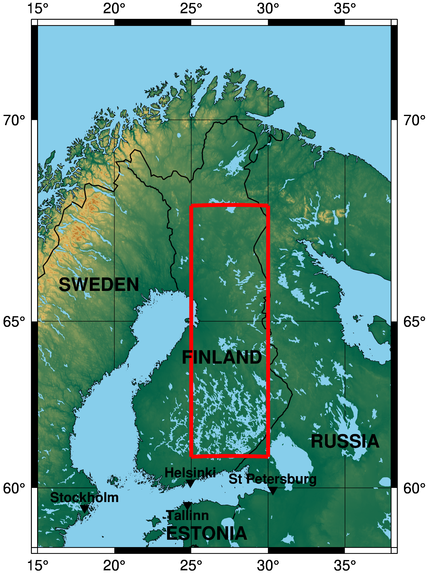
Figure 1The area used in the spatially averaged forecasts in Finland.
The effect of seasonality on the forecast skill was removed by subtracting the first three harmonics of the annual cycle.
2.2 Non-homogeneous Gaussian regression
In this study, NGR was used to correct the mean weekly forecast, not the forecasts at each time step, as in, e.g., Thorarinsdottir and Gneiting (2010) or Baran and Lerch (2016). This simplifies the modelling somewhat; according to the central limit theorem (e.g., Wilks, 2019), the distribution of means will tend to be Gaussian in shape.
NGR provides the Gaussian probability distribution
where μ is the mean, and σ is the standard deviation. In contrast to the regular Gaussian regression, σ is not a constant. The mean μ is
where is the ensemble mean and the standard deviation σ is
where s is the ensemble standard deviation. The constants a, b, c, and d are then fitted (or trained) with the data. The logarithm in Eq. (3) is used to keep the estimated σ positive and is not strictly necessary, but Messner et al. (2016) note that problems in the numerical optimisation can occur if it is not used.
In this study, deterministic forecasts were the mean μ parameter of the NGR. The probabilistic forecasts utilise both the mean and the standard deviation parameters, so both the bias and spread of forecasts are adjusted.
2.3 Verification methods
For the verification terminology, we follow Messner et al. (2016). For the deterministic forecasts, the commonly used measure is the mean squared error (MSE)
where y is the forecast (here the mean μ parameter of the NGR) and o is the observation (here the weekly mean of ERA-Interim). The MSE can be shown as the function of the mean error (ME, ), the standard deviation of observations and forecasts (so and sy), and their Pearson correlation (ryo) (Wilks, 2019)
For the perfect forecast, the MSE should be zero, implying that the ME should be zero, so and sy should be equal, and ryo should be one.
The continuous ranked probability score (CRPS) is used for the probabilistic forecasts
where F(y) and Fo(y) are the cumulative distribution functions of the forecast and the observation. Scores were calculated using the scoringRules package (Jordan et al., 2019). The CRPS can also be decomposed, but published methods (Hersbach, 2000) involve ensemble forecasts, not probability distributions as in this study, so we did not pursue decomposition further.
For a score S, with the best possible score being zero, the general form of a skill score (SS) is
where Sref is the score of the reference forecast. Here skill scores of the MSE (MSESS) and the CRPS (CRPSS) are used with the reference forecasts being climatological forecasts based on the ERA-Interim. The MSESS based on the climatological reference forecasts is comparable to the coefficient of determination (R2) in linear regression (Wilks, 2019).
Now we can define skilful forecasts as forecasts with a skill score higher than zero. And to be more precise, the forecast is skilful at a statistically significant level, if zero is not within confidence intervals (CIs). As we used both Monday and Thursday forecasts, there is autocorrelation in the data, so the effective number of forecasts is not as high as 1000 for each lead time. This must be taken into account when CIs are calculated. Therefore, the CIs of verification measures are calculated with block-bootstrap (e.g., Wilks, 2019). The block size L=15 was used, with L being calculated with the software provided in Patton (2009). The number of bootstrap samples was 5000.
The size of the reforecast ensemble (11 members) is smaller than the size of the climatological ensemble (30 members), and the CRPS values of NGR reforecasts are not readily comparable with the climatological forecasts. Therefore, we used the formula given by Ferro et al. (2008) to estimate the CRPS as if the NGR ensemble would have had the same number of members as climatological forecasts
where m=11 is the original size and M=30 is the new size.
The quality of probabilistic forecasts was also evaluated using the relative operating characteristic (ROC) curves (see, e.g., Wilks, 2019). Here we concentrate on the area under the ROC curve (AUROC) that can be shown as a time series. Values larger than 0.5 show skill, the best value being 1.0. The ROC is often interpreted to show potential skill (Kharin and Zwiers, 2003). We validated the probability of the forecasts of mean winds being greater than the 50th percentile (calculated from the training data set).
3.1 How the NGR changes unadjusted reforecasts
The NGR is not a black box and the change of the constants of Eqs. (2) and (3) as the function of the lead time gives insight into the performance of the method. The coefficient a, the constant of Eq. (2), grows as the lead time increases, while b, the coefficient of the ensemble means, decreases (Fig. 2a). In practice, this means that as the lead time increases the NGR pushes the forecast towards the climatology. In our data set, the range of mean wind observations is roughly from 2 m/s to 5 m/s, the mean being roughly 3.4 m/s. Then, if we calculate fictive forecasts of 2–5 m/s as the function of the lead time (Fig. 2b), we see that the forecasts larger (smaller) than the mean are increasingly reduced (increased) as the lead time increases, so they tend to the climatological mean, about 3.4 m/s.

Figure 2The fitted coefficients for NGR as the function of lead time: (a) the mean (Eq. 2), and (b) how the ensemble mean of the unadjusted or raw forecast is then modified by the NGR. (c) The standard deviation (Eq. 3, using only the intercept term) shown along with the ensemble standard deviation of the unadjusted forecasts and the standard deviation of observations (based on ERA-Interim). To help interpreting the standard deviation values, the logarithm was not used in Eq. (3). The training set, odd winters during 1997–2017, was used.
For the data set here, d of Eq. (3), the coefficient of the ensemble standard deviations was rather noisy and often not statistically significant, and, without any notable change in the results, only the constant c could be used (Fig. 2c). For all lead times, the NGR standard deviation is slightly larger than the unadjusted ensemble spread, and for longer lead times both tend to the standard deviation of the observations (Fig. 2c).
3.2 Verification results
The ME of both NGR adjusted reforecasts and climatological forecasts is nearly zero (Fig. 3a), the zero being inside the CIs. This is encouraging, as the ME of climatological forecasts should be zero, and the very small ME of reforecasts suggests that the NGR succeeds in bias correction.
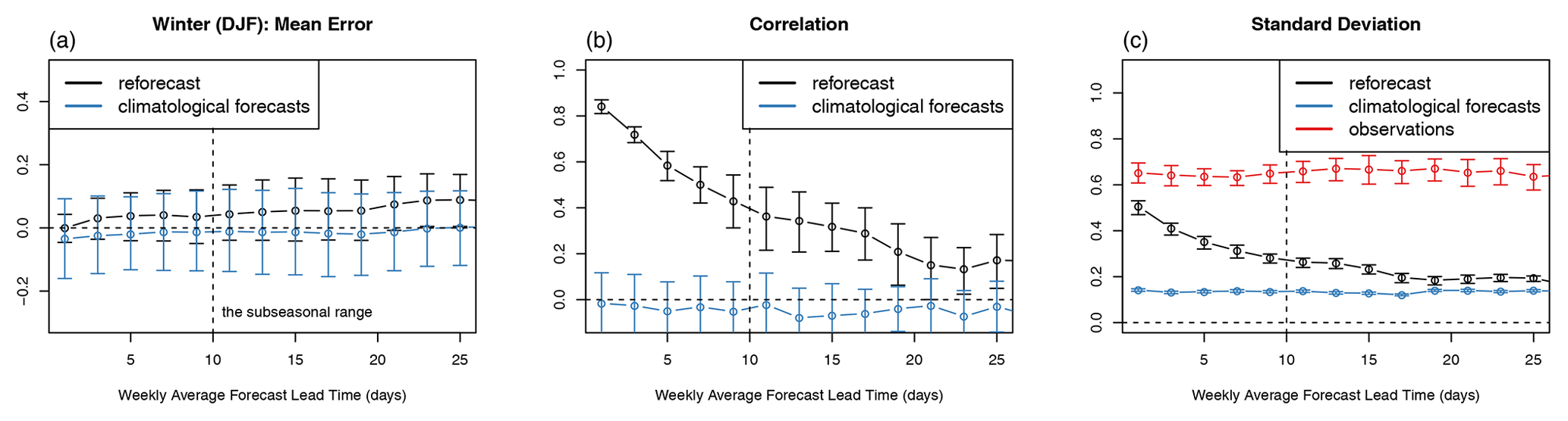
Figure 3The verification measures of reforecasts (using the validation set, even winters 1996–2016) for the averaged area (Fig. 1). Reforecasts are the mean of one week of 6-hourly reforecasts and start every two days. For reforecasts and climatological forecasts, the parts of the MSE decomposition (Eq. 5) are: (a) the mean error, (b) correlation, and (c) standard deviation.
The correlation of NGR reforecasts decreases as the lead time increases but remains positive at the last lead time calculated (Fig. 3b). The correlation of climatological forecasts is zero or slightly negative, but the zero remains encouragingly inside the CIs because climatological forecasts should not have any skill. The standard deviation of NGR reforecasts is almost equal to that of the observations in the first lead time (Fig. 3c), but decreases steadily, even though it remains slightly larger than the standard deviation of climatological forecasts. It is not surprising that the standard deviation of NGR reforecasts decreases from larger values (similar to the observations) to smaller values (similar to climatology), as we have shown how the means of NGR reforecasts tend to climatology (Fig. 2b).
The MSESS remains statistically significantly positive until the lead time of 21 d, when the CI includes zero (Fig. 4a). Skilful weekly forecasts cover almost all of the third week. The original CRPSS (with 11 members in the ensemble) remains statistically positive until the lead time of 19 d (Fig. 4b), while its value is smaller than the MSESS for all lead times. After estimating the CRPS for 30 members by using Eq. (8) (Fig. 4c), the CRPSS remains positive for all lead times. This might not be a sensible result. However, the CRPSS values stabilise after the lead time of 21 d. Therefore, not accounting for the smaller ensemble size might give us too pessimistic a result, but using Eq. (8) might give us a too optimistic a result.

Figure 4The verification measures of reforecasts (using the validation set, even winters 1996–2016) for the averaged area (Fig. 1). Reforecasts are the mean of one week of 6-hourly reforecasts and start every two days. The skill score for (a) the MSE, (b) the CRPS without adjustment, (c) the CRPS adjusted with Eq. (8). (d) The area under ROC for the forecasts of mean winds greater than the 50th percentile.
The AUROC (Fig. 4d) remains higher than 0.5 for all lead times considered here. This is not realistic, and it clearly shows that we were not able to remove the effect of seasonality just by subtracting the first three harmonics. The AUROC stabilises around a lead time of 21 d, so the result is consistent with the MSESS and the CRPSS.
Our results are comparable to those of Lynch et al. (2014), who concluded that there is statistically significant skill in predicting weekly mean wind speeds over areas of Europe at lead times of at least 14–20 d. Lynch et al. (2014) used five years of operational forecasts; their CIs were narrower than ours, and they could make better inference using operational forecasts.
Prior to analysis, we anticipated that the CRPSS (Fig. 4b and c) would have remained skilful longer than the MSESS (Fig. 4a), and the CRPSS would have been higher, because the probabilistic forecasts contain more information than deterministic forecasts. While the MSE and the CRPS values cannot be directly compared, deterministic and probabilistic forecasts can be directly compared using the mean absolute error (MAE) of the deterministic forecasts, because the CRPS reduces to the MAE when the forecast is deterministic. Therefore we calculated the MAE (or the CRPS, as they are equal) of the deterministic forecasts and compared it to the CRPS of the probabilistic climate forecasts, and the MAE was smaller than the climatological CRPS (or the CRPSS is greater than zero) only for the first two lead times (not shown). So, not surprisingly, the probabilistic forecasts do contain more information than the deterministic forecasts, but as the skill scores show, deterministic forecasts are better compared with their reference forecasts. How, then, should we interpret this result? Maybe the deterministic reference forecasts could be improved; therefore, perhaps their skill scores presented here are spuriously high and we should concentrate on probabilistic results for a more realistic skill assessment? Or maybe our probabilistic forecasts could be improved, and meanwhile, the deterministic forecasts show what kind of skill can be achieved in the future? A prudent answer is always to choose the less skilful results, and to not be overconfident.
The use of Eq. (8) should be carefully considered: Ferro et al. (2008) developed the results for discrete ensemble forecasts, and it is unclear how applicable it is when the NGR is used for forecasts. The smaller ensemble size still makes it harder to estimate μ and σ, but is Eq. (8) an applicable estimator for that?
It is also important to further investigate the impact of the seasonal cycle on the verification results, as an uncritical reading of figures might suggest unrealistic trust in the forecasts.
4.1 The usability of wind speed forecasts
The forecasts might be skilful even for the third week, but the skill is still very low, even if the skill scores are non-zero or positive. For example, an MSESS of around 0.1 can be interpreted as 10 % of the variance explained, which is very little for most applications. So it is not straightforward to see who is the potential user that could benefit from the third-week forecasts. Using the categorisation of users by Raftery (2016), we can assume that a casual, low stakes user (“Should I wear a sweater or a short-sleeved shirt?”) might not benefit much from these forecasts, but a user who understands how to use the probabilities in a decision theory framework should be able to utilise the forecasts and benefit from them if they ”play the game” long enough. For the wind forecasts, such a user might be an energy company using renewable energy sources.
In general, the utility of forecasts is defined by the users, so close co-operation and co-development of forecasts with the users is useful, if not essential. Moreover, the mean weekly wind itself might not be useful for most end users. For example, warnings of extreme wind would need percentiles higherthan 50 % (see, e.g., Friederichs et al., 2018) and wind power forecasts would need the whole probability distribution as wind power has a non-linear response to wind speed (Pinson and Messner, 2018).
4.2 Future research
It seems reasonable to assume that different reanalyses generate somewhat different climatologies and observations, implying somewhat different skill scores based on different reanalyses. This is especially relevant for a variable such as wind, which is not so straight-forward to measure. So, the use of more than one reanalysis might be useful in future studies. In this study, we used the ERA-Interim as our reference, but more recent reanalyses, such as MERRA-2 (Gelaro et al., 2017) and ERA5 (Hersbach et al., 2020) (which became available after this project ended), would be natural candidates to be used in further studies.
The bias-adjustment methods used here are only rudimentary and could be improved. For example, Siegert and Stephenson (2019) note that explicit spatiotemporal statistical models are largely unexplored in subseasonal studies. For weather forecasts, Rasp and Lerch (2018) compare NGR with machine learning methods, and show that auxiliary information is needed to improve forecasts. For a subseasonal range in northern America, one source of such information might be indices such as the MJO or ENSO (Vigaud et al., 2018). For Northern Europe, suitable indices might be the QBO (e.g., Kidston et al., 2015) or the strength of the polar vortex (Korhonen et al., 2020). Including such information in NGR is rather straight-forward. Furthermore, the most advanced non-linear methods (such as deep learning, e.g., Liu et al., 2016) need a large amount of training data to avoid overfitting, and the data sets available in subseasonal forecasting are of relatively modest size. Therefore, NGR, trainable with reasonable small data, is a feasible choice for future applications.
We evaluated the weekly mean wind forecasts for Finland based on the ECMWF forecasts. The NGR was used to correct the reforecasts. The skill of forecasts appears to be positive for the third week, but the longest skilful lead time depends on the reference data sets, the scores used, and the correction methods. Also, two winters would have been a rather short time span to make meaningful inferences on how operational wind forecasts perform, so reforecasts with longer time span are essential for comparison. Even then some uncertainty remains. The needs and the competence of the end users determine whether the forecasts are useful or not. The forecasts would be most beneficial for users applying the probabilities in the decision theory framework.
The ECMWF reforecasts and ERA-Interim are available for the national meteorological services of ECMWF member and co-operating states and holders of suitable licences.
OH did most of the analysis and wrote most of the article. TKL wrote parts of the Introduction and contributed to the preparation of the paper. OR contributed to the statistical analysis. NK and VA contributed to the preparation of the paper. GH supervised the project.
The author declares that there is no conflict of interest.
Publisher’s note: Copernicus Publications remains neutral with regard to jurisdictional claims in published maps and institutional affiliations.
This article is part of the special issue “Applied Meteorology and Climatology Proceedings 2020: contributions in the pandemic year”.
We thank Jussi Ylhäisi for the helpful comments on the early draft of this paper.
This research has been supported by the Academy of Finland (grant nos. 303951 and 321890).
This paper was edited by Andrea Montani and reviewed by two anonymous referees.
Baran, S. and Lerch, S.: Mixture EMOS model for calibrating ensemble forecasts of wind speed, Environmetrics, 27, 116–130, https://doi.org/10.1002/env.2380, 2016. a
Buizza, R. and Leutbecher, M.: The forecast skill horizon, Q. J. Roy. Meteor. Soc., 141, 3366–3382, https://doi.org/10.1002/qj.2619, 2015. a
Dee, D. P., Uppala, S. M., Simmons, A. J., Berrisford, P., Poli, P., Kobayashi, S., Andrae, U., Balmaseda, M. A., Balsamo, G., Bauer, P., Bechtold, P., Beljaars, A. C. M., van de Berg, L., Bidlot, J., Bormann, N., Delsol, C., Dragani, R., Fuentes, M., Geer, A. J., Haimberger, L., Healy, S. B., Hersbach, H., Hólm, E. V., Isaksen, L., Kållberg, P., Köhler, M., Matricardi, M., McNally, A. P., Monge-Sanz, B. M., Morcrette, J.-J., Park, B.-K., Peubey, C., de Rosnay, P., Tavolato, C., Thépaut, J.-N., and Vitart, F.: The ERA-Interim reanalysis: configuration and performance of the data assimilation system, Q. J. Roy. Meteor. Soc., 137, 553–597, https://doi.org/10.1002/qj.828, 2011. a
ECMWF: IFS documentation, CY43R2, Part V: Ensemble Prediction System, ECMWF, available at: https://www.ecmwf.int/sites/default/files/elibrary/2016/17118-part-v-ensemble-prediction-system.pdf (last access: 2 August 2021), 2016. a
Ervasti, T., Gregow, H., Vajda, A., Laurila, T. K., and Mäkelä, A.: Mapping users' expectations regarding extended-range forecasts, Adv. Sci. Res., 15, 99–106, https://doi.org/10.5194/asr-15-99-2018, 2018. a
Ferro, C. A. T., Richardson, D. S., and Weigel, A. P.: On the effect of ensemble size on the discrete and continuous ranked probability scores, Meteorol. Appl., 15, 19–24, https://doi.org/10.1002/met.45, 2008. a, b
Friederichs, P., Wahl, S., and Buschow, S.: Postprocessing for Extreme Events, in: Statistical Postprocessing of Ensemble Forecasts, edited by: Vannitsem, S., Wilks, D., and Messner, J., Elsevier, Amsterdam, 2018. a
Gelaro, R., McCarty, W., Suárez, M. J., Todling, R., Molod, A., Takacs, L., Randles, C. A., Darmenov, A., Bosilovich, M. G., Reichle, R., Wargan, K., Coy, L., Cullather, R., Draper, C., Akella, S., Buchard, V., Conaty, A., da Silva, A. M., Gu, W., Kim, G.-K., Koster, R., Lucchesi, R., Merkova, D., Nielsen, J. E., Partyka, G., Pawson, S., Putman, W., Rienecker, M., Schubert, S. D., Sienkiewicz, M., Zhao, B., Gelaro, R., McCarty, W., Suárez, M. J., Todling, R., Molod, A., Takacs, L., Randles, C. A., Darmenov, A., Bosilovich, M. G., Reichle, R., Wargan, K., Coy, L., Cullather, R., Draper, C., Akella, S., Buchard, V., Conaty, A., da Silva, A. M., Gu, W., Kim, G.-K., Koster, R., Lucchesi, R., Merkova, D., Nielsen, J. E., Partyka, G., Pawson, S., Putman, W., Rienecker, M., Schubert, S. D., Sienkiewicz, M., and Zhao, B.: The Modern-Era Retrospective Analysis for Research and Applications, Version 2 (MERRA-2), J. Climate, 30, 5419–5454, https://doi.org/10.1175/JCLI-D-16-0758.1, 2017. a
Gneiting, T., Raftery, A. E., Westveld, A. H., and Goldman, T.: Calibrated Probabilistic Forecasting Using Ensemble Model Output Statistics and Minimum CRPS Estimation, Mon. Weather Rev., 133, 1098–1118, https://doi.org/10.1175/MWR2904.1, 2005. a
Hersbach, H.: Decomposition of the Continuous Ranked Probability Score for Ensemble Prediction Systems, Weather Forecast., 15, 559–570, https://doi.org/10.1175/1520-0434(2000)015<0559:DOTCRP>2.0.CO;2, 2000. a
Hersbach, H., Bell, B., Berrisford, P., Hirahara, S., Horányi, A., Muñoz‐Sabater, J., Nicolas, J., Peubey, C., Radu, R., Schepers, D., Simmons, A., Soci, C., Abdalla, S., Abellan, X., Balsamo, G., Bechtold, P., Biavati, G., Bidlot, J., Bonavita, M., Chiara, G., Dahlgren, P., Dee, D., Diamantakis, M., Dragani, R., Flemming, J., Forbes, R., Fuentes, M., Geer, A., Haimberger, L., Healy, S., Hogan, R. J., Hólm, E., Janisková, M., Keeley, S., Laloyaux, P., Lopez, P., Lupu, C., Radnoti, G., Rosnay, P., Rozum, I., Vamborg, F., Villaume, S., and Thépaut, J.: The ERA5 Global Reanalysis, Q. J. Roy. Meteor. Soc., 146, 1999–2049, https://doi.org/10.1002/qj.3803, 2020. a
Jordan, A., Krüger, F., and Lerch, S.: Evaluating Probabilistic Forecasts with scoringRules, J. Stat. Softw., 90, 12, https://doi.org/10.18637/jss.v090.i12, 2019. a
Kharin, V. V. and Zwiers, F. W.: On the ROC Score of Probability Forecasts, J. Climate, 16, 4145–4150, https://doi.org/10.1175/1520-0442(2003)016<4145:OTRSOP>2.0.CO;2, 2003. a
Kidston, J., Scaife, A. A., Hardiman, S. C., Mitchell, D. M., Butchart, N., Baldwin, M. P., and Gray, L. J.: Stratospheric influence on tropospheric jet streams, storm tracks and surface weather, Nat. Geosci., 8, 433–440, https://doi.org/10.1038/NGEO2424, 2015. a
Korhonen, N., Hyvärinen, O., Kämäräinen, M., Richardson, D. S., Järvinen, H., and Gregow, H.: Adding value to extended-range forecasts in northern Europe by statistical post-processing using stratospheric observations, Atmos. Chem. Phys., 20, 8441–8451, https://doi.org/10.5194/acp-20-8441-2020, 2020. a
Liu, Y., Racah, E., Prabhat, Correa, J., Khosrowshahi, A., Lavers, D., Kunkel, K., Wehner, M., and Collins, W.: Application of Deep Convolutional Neural Networks for Detecting Extreme Weather in Climate Datasets, arXiv [preprint], arXiv:1605.01156 (last access: 2 August 2021), 2016. a
Lynch, K. J., Brayshaw, D. J., and Charlton-Perez, A.: Verification of European Subseasonal Wind Speed Forecasts, Mon. Weather Rev., 142, 2978–2990, https://doi.org/10.1175/MWR-D-13-00341.1, 2014. a, b, c, d
Matsueda, M. and Nakazawa, T.: Early warning products for severe weather events derived from operational medium-range ensemble forecasts, Meteorol. Appl., 22, 213–222, https://doi.org/10.1002/met.1444, 2015. a
Messner, J. W., Mayr, G. J., and Zeileis, A.: Heteroscedastic Censored and Truncated Regression with crch, R J., 8, 173–181, https://doi.org/10.32614/RJ-2016-012, 2016. a, b, c
Neal, R. A., Boyle, P., Grahame, N., Mylne, K., and Sharpe, M.: Ensemble based first guess support towards a risk-based severe weather warning service, Meteorol. Appl., 21, 563–577, https://doi.org/10.1002/met.1377, 2014. a
Patton, A.: Correction to “Automatic Block-Length Selection for the Dependent Bootstrap” by D. Politis and H. White, Economet. Rev., 28, 372–375, https://doi.org/10.1080/07474930802459016, 2009. a
Pinson, P.: Wind Energy: Forecasting Challenges for Its Operational Management, Stat. Sci., 28, 564–585, https://doi.org/10.1214/13-STS445, 2013. a
Pinson, P. and Messner, J. W.: Application of Postprocessing for Renewable Energy, in: Statistical Postprocessing of Ensemble Forecasts, edited by: Vannitsem, S., Wilks, D., and Messner, J., Elsevier, Amsterdam, 2018. a
Raftery, A. E.: Use and communication of probabilistic forecasts, Stat. Anal. Data Min., 9, 397–410, https://doi.org/10.1002/sam.11302, 2016. a
Rasp, S. and Lerch, S.: Neural Networks for Postprocessing Ensemble Weather Forecasts, Mon. Weather Rev., 146, 3885–3900, https://doi.org/10.1175/MWR-D-18-0187.1, 2018. a
Siegert, S. and Stephenson, D. B.: Forest Recalibration and Multimodel Combination, in: Subseasonal to Seasonal Prediction Project: the gap between weather and climate forecasting, edited by: Robertson, A. W. and Vitart, F., Elsevier, Amsterdam, 2019. a
Thorarinsdottir, T. L. and Gneiting, T.: Probabilistic forecasts of wind speed: ensemble model output statistics by using heteroscedastic censored regression, J. Roy. Stat. Soc. Ser. A, 173, 371–388, https://doi.org/10.1111/j.1467-985X.2009.00616.x, 2010. a
Toth, Z. and Buizza, R.: Weather forecasting: what sets the forecast skill horizon?, in: Sub-seasonal to seasonal prediction: the gap between weather and climate forecasting, edited by: Robertson, A. W. and Vitart, F., Elsevier, Amsterdam, 2018. a
Vigaud, N., Robertson, A., and Tippett, M. K.: Predictability of Recurrent Weather Regimes over North America during Winter from Submonthly Reforecasts, Mon. Weather Rev., 146, 2559–2577, https://doi.org/10.1175/MWR-D-18-0058.1, 2018. a
Vitart, F.: Evolution of ECMWF sub-seasonal forecast skill scores, Q. J. Roy. Meteor. Soc., 140, 1889–1899, https://doi.org/10.1002/qj.2256, 2014. a, b
White, C. J., Carlsen, H., Robertson, A. W., Klein, R. J., Lazo, J. K., Kumar, A., Vitart, F., Coughlan de Perez, E., Ray, A. J., Murray, V., Bharwani, S., MacLeod, D., James, R., Fleming, L., Morse, A. P., Eggen, B., Graham, R., Kjellström, E., Becker, E., Pegion, K. V., Holbrook, N. J., McEvoy, D., Depledge, M., Perkins-Kirkpatrick, S., Brown, T. J., Street, R., Jones, L., Remenyi, T. A., Hodgson-Johnston, I., Buontempo, C., Lamb, R., Meinke, H., Arheimer, B., and Zebiak, S. E.: Potential applications of subseasonal-to-seasonal (S2S) predictions, Meteorol. Appl., 24, 315–325, https://doi.org/10.1002/met.1654, 2017. a
Wilks, D. S.: Comparison of ensemble-MOS methods in the Lorenz '96 setting, Meteorol. Appl., 13, 243, https://doi.org/10.1017/S1350482706002192, 2006. a
Wilks, D. S.: Statistical Methods in the Atmospheric Sciences, 4 edn., Elsevier, Amsterdam, 2019. a, b, c, d, e