 | 01 Jun 2022
Predictability analysis and skillful scale verification of the Lightning Potential Index (LPI) in the COSMO-D2 high resolution ensemble system
Michele Salmi
Chiara Marsigli
Manfred Dorninger
During the last decade, the constant improvement in computational capacity led to the development of the first limited-area, kilometer-scale ensemble prediction systems (L-EPS). The COSMO-D2 EPS (now ICON-D2) was the operational L-EPS at the German weather service (DWD) and has a spatial resolution of around 2.2 km. This grid resolution allows large scale, deep convective processes such as thunderstorms or heavy showers to be handled explicitly, without any physical parametrization. Special parameters involving both clouds microphysics and large scale lifting – such as the Lightning Potential Index, or LPI – have also been developed in order to try to bring the forecasting of deep convection and therefore also of lightning activity to a new level of spatial accuracy. With such high resolution forecasts comes however also a higher error potential, at least for gridpoint-verification. The use of this high resolution setup in an ensemble prediction system might however bring huge benefits in terms of skill and predictability. This work is a preliminary attempt to apply innovative verification approaches such as the dispersion Fractions Skill Score (dFSS) and the ensemble-SAL (eSAL) to the LPI in the COSMO-D2 EPS. Aim of this work is to assess the relationship between the ensemble error and the ensemble dispersion at different spatial scales. For the summer months 2019, the COSMO-D2 EPS shows a general tendency to overestimate the predictability (underestimate the ensemble spread) of the lightning events, though the spread-error relationship varies greatly for different forecast lead times. With the help of the dFSS, one can also express this relationship in terms of skillful scales. On average, the system produces a useful forecast during the afternoon hours for horizontal scales of around 200 km. However, the ensemble members show an average horizontal dispersion that amounts to around half of that value, at more or less 100 km.
- Article
(3811 KB) - Full-text XML
- BibTeX
- EndNote


The forecast of convective activity is one of the most challenging topics in weather modeling, as convective cells are typically localized in time and space and can be significantly driven by small scale processes, which includes turbulence and cloud microphysics. At the same time, convection can cause very high human and economic losses as it is often accompanied by hail, flash floods or severe wind gusts. Due to the electrical charge separation that takes place in the convective cloud (Saunders, 2008), lightning strikes are the most typical phenomena that accompany convection and are themselves sources of significant injuries to people and damages to properties. An accurate forecast of deep convection brings therefore huge benefits in terms of assessing the likelihood of potentially severe weather. For many years however, convection has been a sub-grid phenomenon in weather models that needed to be parametrized because of their poor spatial resolution. It was not until recently that the most advanced local area models reached a grid spacing on the lower end of the mesoscale, close to the kilometer-scale, allowing deep convection to be handled explicitly.
Following such improvements, in the last decade the first parameters aiming at forecasting the lightning activity came along (McCaul et al., 2009), with the Lightning Potential Index (LPI) (Lynn and Yair, 2010; Lynn et al. , 2012) being one of the first to be developed and tested in the framework of the Weather Research and Forecasting model (WRF). Parallel to this evolution and thanks to the constantly improving computational capacity, also the first convection-permitting ensemble prediction systems (EPS) have emerged. In Europe, the COSMO-Consortium (https://www.cosmo-model.org/, last access: 28 May 2022) started developing its version of high resolution EPS already in the early 2000s with the COSMO-LEPS system (Montani et al., 2003). In the last decade, convection-permitting ensembles have been developed in several countries, the first being COSMO-DE-EPS (Gebhardt et al., 2011). The system, now ICON-D2-EPS, has 20 members with 2.2 km horizontal resolution and is maintained by the German Weather Service (DWD). Starting from 2015, the LPI has also been adapted for the COSMO-D2 EPS (Blahak, 2015) and has been routinely included in its output fields. The COSMO-LPI approach is particularly interesting, as the parameter mixes the microphysical properties of the cloud – such as the liquid water to ice water ratio – with some large scale lifting parameters in order to provide an ultra-fine forecast of lightning activity.
After half a decade though, only little research has been conducted on how this innovative way of forecasting convection is performing in the framework of a very high resolution probabilistic model. This work aims at raising attention to this field and is a preliminary attempt at assessing the skill and the predictability of lightning activity in an high resolution EPS. In order to achieve this, it makes use of some well established, neighbourhood and object-based verification methods such as the Fractions Skill Score, or FSS (Roberts and Lean, 2008) and the Structure-Amplitude-Location, or SAL (Wernli et al., 2008). Their probabilistic form, the dispersion FSS, here referenced to as dFSS (Dey et al., 2014) and the ensemble SAL, or eSAL (Radanovics et al., 2018) are being proposed for a spread-skill evaluation of the ensemble forecast of convection in terms of LPI. Is the high resolution, probabilistic approach of a L-EPS leading to some benefits in forecasting convection in general and lightning activity in particular? Furthermore, do the proposed verification metrics give detailed insights and information about the quality of the forecast?
In this work, the COSMO-D2 EPS model forecasts for the summer months (JJA) 2019 have been verified against observational data coming from the LIghtning detection NETwork (LINET) provided by the German Weather Service (DWD).
2.1 Observations – LINET lightning detection network
The LINET network (Betz et al., 2004, 2009) is one of the best performing lightning detection networks covering Central Europe. Around 100 Very Low Frequency/Low Frequency (VLF/LF) sensors detect the variations in the electromagnetic spectrum caused by lightning strikes and are able to localize them using an optimized Time Of Arrival algorithm (TOA). This setup ensures an average accuracy of around 150 m (Karagiannidis et al., 2019), which is one order of magnitude higher than the COSMO-D2 horizontal resolution (see next section) and therefore more than acceptable for this study. The network is also able to determine the height of the intracloud discharges, but this feature has not been used in this work. A list of detected lightning strokes with very precise values for latitude, longitude and time of occurrence over Central Europe has been compiled for the summer 2019 and then transferred onto the model grid. A simple nearest neighbor method has been used to sum up all the lightning strokes occurring inside a COSMO-D2 model grid box during a 1 h time window. Data falling outside of the model domain has been rejected. The resulting datasets are gridded observed number of lightning strokes on a hourly basis, covering the summer months of 2019 and corresponding to the COSMO-D2 grid (Fig. 1). The available raw data are quality controlled and therefore no further filtering or quality check has been applied.
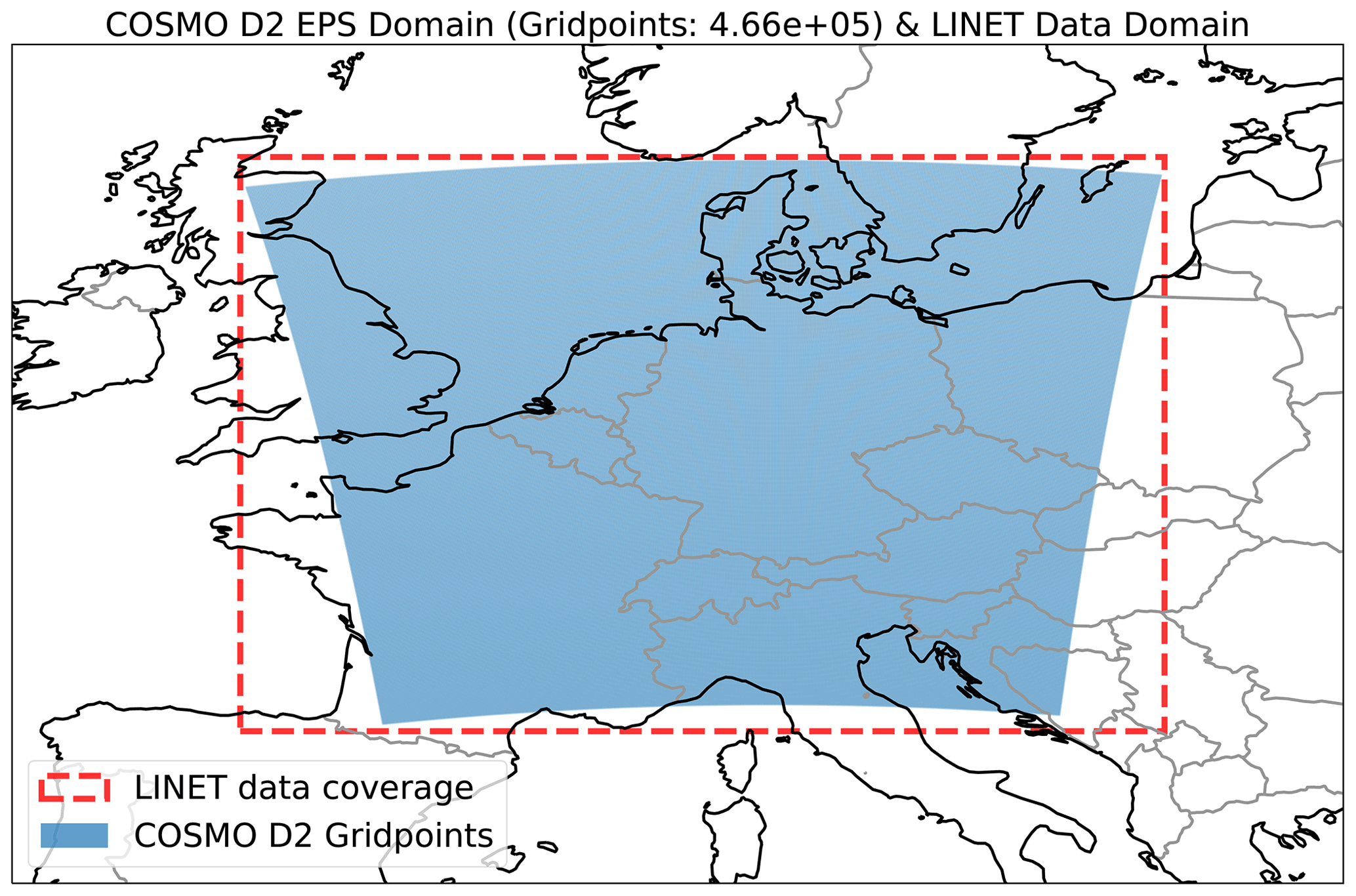
Figure 1COSMO-D2 EPS domain (blue area) and LINET data coverage (red rectangle).
2.2 Forecasts – COSMO-D2 EPS lightning potential index
The COSMO-D2 EPS fields used in this work are based on the DWD's model chain setup of 2019. A global model provides both deterministic (ICON) and probabilistic (ICON-EPS) forecasts with respectively 13 and 40 km – 6.5 and 20 km for the European domain refinement (ICON-EU and ICON-EU-EPS) – horizontal grid spacing. The probabilistic model, ICON-EPS, calculates 40 different perturbed members. These fields provide the boundary conditions for a 2.2 km nested model for central Europe named COSMO-D2 (more on the COSMO model at: https://www.cosmo-model.org/, last access: 28 May 2022). The high resolution model, COSMO-D2, has 65 vertical levels and can handle deep convective processes explicitly. Shallow convection as well as cloud microphysics are still sub-grid processes that need a specific parametrization scheme and closure. For the cloud microphysics, a 6-classes parametrization scheme that includes the category “graupel” is applied. A detailed description of both the global and the local model can be found on the DWD's website (Baldauf et al., 2018; Reinert et al., 2021). The probabilistic, high resolution twin model is called COSMO-D2 EPS and is physically identical to the deterministic version. The initial conditions of the 20 different ensemble members are provided by the Kilometre-scale ENsemble Data Assimilation (KENDA) scheme, based on an ensemble-Kalman-filter, developed specifically for the COSMO Consortium (Schraff et al., 2016). Furthermore, randomized basic perturbations are applied to the physics of the model, including convective processes. Finally, the boundary conditions for the 20 members are obtained from the ICON-EU-EPS model.
The Lightning Potential Index or LPI (Lynn and Yair, 2010; Lynn et al. , 2012) assesses the energy available for charge separation inside the convective cloud and is therefore measured in J kg−1. The formula that defines the LPI takes into account the strength of the updraft w and the liquid water to ice water ratio in the relevant portion of the cloud where electrification typically occurs (between the heights and ). Starting from 2015, an adapted version of the LPI with some additional boolean functions (Blahak, 2015) has been included in the COSMO-D2 EPS model as defined in Eq. (1).
In particular, f1 is a boolean function that investigates the average strength of the updrafts in a square of 10 km around the grid point. If the maximum updraft is weaker than 1.1 m s−1 over more than half of the square, then f1 takes the value 0, otherwise it switches to 1. In the same way, f2 is 0 when the average convective buoyancy available over a square of 20 km around the grid point does not reach a specific threshold. Both functions are introduced in order to filter out false alarms when convection is expected to be relatively shallow or mostly single-celled, which lowers the potential for lightning strikes. Furthermore, g(w) filters out (i.e. is equal to 0) all the vertical levels where the updraft velocity is weaker than 0.5 m s−1 and is 1 in all other cases. Finally, ϵ is a dimensionless function that can take values between 0 and 1 and is defined as:
where Ql and Qs are the total liquid water mass mixing ratio and the ice fractional mixing ratio that includes graupel, snow and hail (both kg kg−1) respectively. Basically, ϵ is maximized when the amount of (supercooled) liquid water and the ice portion in the convective cloud are equal. If one of the two parts is close to one (either liquid or solid water), ϵ tends to zero. This is where the LPI takes into account the microphysical properties of the cloud for each of the model vertical levels in order to assess the potential for charge separation to occur.
The COSMO-D2 EPS LPI fields for the 20 ensemble members are originally made available with a 15 min forecast step. In order to reduce the computational resources necessary to process the whole dataset, the time frequency has been reduced from 15 min to 1 h by taking the maximum of the LPI in each time window. The forecasts cover 1.125 d with a forecast length of 27 h and there is a new model run every 3 h. For this work, just the 00:00 UTC runs and only the first 24 h lead times in each run have been considered. Over Central Europe, this leads to the following side effect: the hourly forecast steps coincide with the solar time +1 h. This is an important aspect to consider when verifying convective activity, as most of the time it is strongly coupled to daytime heating. The direct consequence of this is that the vast majority of the observed lightning (more than 80 % of the strokes in the dataset) are populating only the forecast steps between +12 and +20 h. As already mentioned, the analysis covers the summer months (June, July, August) of 2019.
As the time of the day plays a central role in the convective cycle, this analysis has been conducted for each hourly forecast step available after reshaping and reorganizing the data. Therefore, all the verification scores presented below provide 24 different values, one for each forecast step, which coincides with the hours of the day, as previously described. Furthermore, as the temporal domain covers the three summer months, for each forecast step a total of 92 d and therefore also a total of 92 model runs is available. See Sect. 3.3 for further details.
As the analysis has been done on a high resolution EPS for rare and extremely localized events such as lightning strikes, the choice of the verification approach is critical. Given these premises and in order to address all the requirements, a neighbourhood verification method, the Fractions Skill Score (FSS) and an object-oriented one, the Structure-Amplitude-Location (SAL) has been adapted for this specific case.
3.1 FSS and dFSS
Very high resolution forecasts can represent meteorological processes and features in a much more realistic way compared to models with coarse resolution, especially when it comes to forecasting convection. However, this does not necessarily lead to better scores when using grid-point verification. Double-penalty issues (Rossa et al., 2008) and the fact that localization errors from parent models are passed over to nested ones can lead to lower skills for high resolution forecasts. In order to address such distortions, fuzzy verification methods have been developed and introduced successfully during the last decades. One of the most successful examples is for sure the Fractions Skill Score, or FSS (Roberts and Lean, 2008), which is defined as the comparison of the Mean Square Error (MSE) with the largest possible MSE (MSE(ref)) over a specific subset of the domain with varying dimension n.
By letting the spatial window size n increase, one can account for possible double-penalty distortions and verify at which spatial scale the high resolution model is reaching a useful skill. The FSS varies between 0 and +1, with 1 being the perfect match between the two fields. According to Roberts and Lean (2008), a forecast field at scale n is defined useful when with f0 being the base rate. The two datasets A and B being compared with the FSS must be binary fields, typically referring to a forecast dataset and an observational one exceeding a predetermined value. In fact, in order to convert the fields in binary form, a significant threshold has to be selected for each field. In our case, however, the two datasets have different measurement units. It would have been possible to convert the forecasts into flash counts using a parametrisation scheme, but such methods can lead to a large mismatch (McCaul et al., 2009). Our goal has been not to modify the original data, whenever possible. Thus, after conducting a previous statistical analysis that also involved a more conventional verification score, the Symmetric Extremal Dependence Index or SEDI (Ferro and Stephenson, 2011) and after looking at different FSS scores for different values of the LPI and the LINET lightning, the optimal thresholds for this study has been defined by:
When it comes to probabilistic forecasts, the FSS can be applied in two different ways. On the one hand it can be used in a conventional way by comparing the observations A with the ensemble mean forecasts B (LeDuc and Hiromu, 2013). In this work, this version of the FSS is called error FSS or eFSS and it addresses the spatial skill of the system. The resulting, total eFSS for each forecast step will be the average of all the eFSS values calculated for each day in the dataset. On the other hand, one can take two members of the ensemble as A and B, obtaining a FSS value from two forecast fields. By applying this to all the ensemble members and then averaging, a measure which is directly related to the spatial spread of the ensemble can be obtained. Therefore, in this study this second version of the FSS is called dispersion FSS or dFSS (Dey et al., 2014). The resulting, total dFSS for each forecast step will then be the average of all dFSS values calculated for each day and each couple of ensemble members in the dataset. This method aggregates the single components of the FSS before averaging. Note that this is not always the best choice, depending on each specific case (Mittermaier et al., 2021). eFSS and dFSS can be directly compared and as the dimension of the subdomain n varies, they provide an additional dimension – the spatial scale – to the classical spread-error relationship analysis. The higher the dFSS, the more alike the ensemble members are (less spread). On the contrary, a lower dFSS means that the ensemble members are less alike (higher spread). Finally, in order to speed up the calculation, all eFSS and dFSS algorithms have been developed using the summed area table or integral image method (Faggian et al., 2015), which optimizes the way each fraction is calculated.
3.2 SAL and eSAL
Another method that goes beyond basic grid-point verification is the object-based Structure-Amplitude-Location (SAL) (Wernli et al., 2008). Key of the SAL is the individuation of single targets or objects within the domain. SAL is composed of three different parts: the structure component S investigates the shape and volume of the objects, the amplitude part A analyzes the overall magnitude of all the objects in the domain and the location component L compares the centers of mass of each identified object and the center of mass of the whole domain to give a measure of spatial skill. In this study, the threshold that defines a SAL-object is set to 1 lightning strike over the whole domain for each grid point. Two (or more) adjacent grid points with contiguous values above 1 are therefore considered as one object. The S and A components can take values between −2 and +2, with 0 being the best performing result. The L component consists of the difference between the domain-wide center of mass plus the difference between the centers of mass of all the objects in the domain and the domain-wide center of mass. Both terms vary between 0 and +1. If both are equal to 0, then the two fields perfectly match in terms of centers of mass.
The SAL has proven to be particularly effective for studying precipitation fields from high resolution models as it takes into account the shape and the spatial distribution of the targets in the domain. Therefore, this method seems to be appropriate also for lightning activity. The adaptation of the SAL for probabilistic forecasts (ensemble SAL or eSAL) has already been documented for precipitation fields (Radanovics et al., 2018; Marsigli et al., 2019). In our case however, the objects of the study originate from two different parameters using different units: the observed number of strokes and the LPI. This makes some further adaptations necessary. Most importantly, the LPI forecast fields need to be translated into number of strokes. In order to achieve this, the exponential function has been used for a curve fitting process. The parameters a, b and c have been optimized using a non-linear least squares regression analysis for each forecast step. In this study, the curve fitting process is based on the same dataset that is being analyzed. Ideally, a different time window should be used to train the curve fitting model. However, a differentiated curve fitting process has been conducted for each week and each month of the dataset, showing only little change in the fitting parameters for different time frames. This supports the hypothesis that in this case the curve fitting process is only weakly sensitive to the chosen data sample. Finally, the LPI fields have been translated to strokes. In order to avoid distortions and be coherent with the thresholds used for the FSS analysis (see Eq. 3), the translated fields have been set to zero a priori for LPI values below 1 J kg−1 being passed to the fitting function.
As for the eFSS/dFSS, also for the SAL it is possible to conduct a classical forecast against observation analysis, or use two forecast fields from two ensemble members in order to investigate the ensemble spread. In this case, the method described by Wernli et al. (2008) is modified only for the fact that an ensemble average SAL – i.e. the mean of 190 SAL values resulting from the comparison of all possible pairs of the 20 members of the EPS – for each model run is being calculated. The reference equations of the ensemble SAL (eSAL) are described in Radanovics et al. (2018), with only the Structure component being calculated differently. For two ensemble members C and D, the analysis has been conducted as follows and then averaged over the ensemble:
where is the sum over the whole list of M detected objects in the domain, while is the sum of the values for each grid point inside each object. Cmax and Dmax are the maximum values inside a single object for the two fields.
3.3 Data filtering
It is well known that lightning are very localized events both in time and space. This is true also for convection in general. In order to focus this analysis on truly active convective days, a general data filtering affecting both the FSS and the SAL analysis has been conducted. For each forecast step, the domain-wide average number of grid points with at least one observed lightning strike LS(Avg) has been calculated. If the average for a specific day is smaller than , this day is omitted from the study. This results on average to halve the number of days processed for each forecast step. As the filtering method is based only on the observed fields, there is the risk of introducing a fictitious bias into the analysis. However, in this case the filtering process retains around 90 % of both the observed and the forecasted lightning activity. Furthermore, the statistics of the False Alarm Rate (FAR) for the filtered and the unfiltered dataset shows changes in the range 0.1 % to 1 % of the FAR, with absolute values ranging between 0.85 and 0.90 depending on the forecast step.
Furthermore, the SAL verification method is inherently object-oriented. In order to prevent large areas of the domain without lightning activity to slightly distort the results (especially for the Location component), a further sub-setting method has been applied prior to the eSAL algorithm. For each day in the dataset, the maximum and minimum latitude and longitude values of the grid points with observed lightning activity has been extrapolated. In the next step, the full domain has been downsized with a zooming function in order to include only the areas with active convection. A buffer of 20 gridpoints (around 45 km) in each geographical direction has been allowed in order to include possible location errors in the forecast as well as possible lightning striking far away from the originating convective cloud. As a result, the analysed domain using SAL changes from hour-to-hour, without affecting the ability to detect large displacement errors.
Figure 2 shows eFSS (Fig. 2a) and dFSS (Fig. 2b) for all forecast steps from +1 to +24 h and for varying neighborhood sizes n from one grid mesh (2.2×2.2 km2) up to 500×500 grid points (around 1100×1100 km2). The white line denotes values that are equal to 0.5, as in this case is extremely small throughout the dataset. Therefore, this line approximately identifies the first spatial scale delivering an acceptable skill. This analysis conveys several useful information. First of all, the dFSS values are overall slightly higher that those of the eFSS, regardless of the neighborhood size or the forecast step. This means that the EPS is generally underdispersive and that the members of the ensemble are not diverging enough to fully represent the spatial uncertainty in the forecast. However, during the time window with most of the lightning activity (i.e. between +14 and +19 h) the spread-error relationship is improving compared to other lead times.
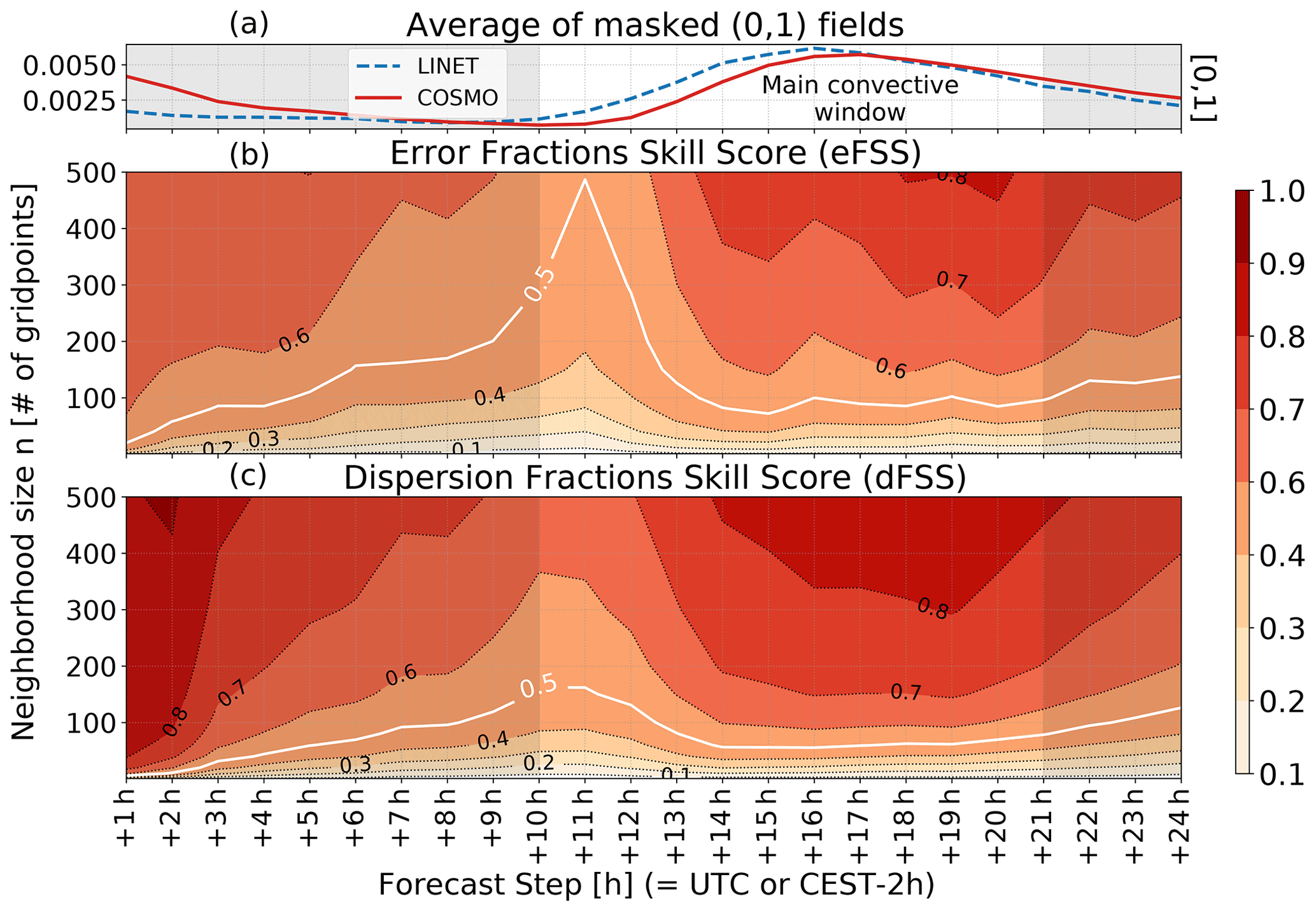
Figure 2(b) Error Fractions Skill Score (eFSS) for 24 forecast steps and neighborhood sizes up to 500 grid points. An eFSS value of is considered as skillful. As is extremely small in this case, the 0.5 line has been highlighted for better reference. (c) Dispersion Fractions Skill Score (dFSS) for 24 hourly forecast steps and neighborhood sizes up to 500 grid points. For COSMO-D2, 1 grid mesh equals 2.2×2.2 km2. For better reference, (a) is showing the average of all the masked fields used for the study (i.e., the average fraction of the domain with observed/forecasted lighting activity), with a clear maximum of the convective activity during the afternoon and evening hours.
Another very interesting feature is the sudden and evident lack of spatial skill occurring at around +11h. The eFSS is basically dropping to a no-skill level even for extremely large neighborhood sizes, which means that there is a significant bias in the model. However, this apparent spatial bias is in fact a timing offset. Looking at the hourly distribution of the LINET flashes and of the LPI values, it is evident that this lack of skill is occurring at the beginning of the diurnal convective cycle. This leads to the conclusion that the model is wrongly delaying the start of the first thundery cells of about 1 h, as the skill then quickly improves again in the early afternoon hours. However, the dFSS analysis is also showing the same drop at around the same time, meaning that the members of the ensemble are diverging more as well and the EPS is likely able to catch some of this lack of predictability. In other words, at least some of the members of the ensemble are likely able to correctly forecast an earlier start of the convective cycle. Even if the magnitude of the drop is not matching the one in the eFSS plot, this is probably signaling that the EPS is able to produce more spread also in case of time related biases. In order to confirm this hypothesis however, further studies with focus on this time window should be conducted.
Concerning the skillful scale presented by the white line on the eFSS plot in Fig. 2, it is interesting to note that this is located at around the 100 grid points scale (220 km) during the afternoon hours, corresponding to the peak hours of lightning activity. On the other hand, the EPS is producing a spatial spread that covers on average half of that value (). This means that the ensemble is overconfident, being too sure to deliver a skillful forecast of lightning activity already at around 50 grid points (or 110 km).
In Fig. 3 the eFSS and dFSS scores for all neighborhood sizes for just four selected forecast steps (+2, +8, +13 and +16 h) are shown. These four steps have been chosen to investigate the spread-error relationship at the beginning of the model run, at the beginning of the main convective window and when lightning activity reaches its daily peak. One should keep in mind that the total eFSS and dFSS values presented in Fig. 2 are actually averages over the whole summer period. However, the eFSS and dFSS values can vary a lot on a day to day basis and for the dFSS also on a member to member basis. For this reason, Fig. 3 also includes the 20th and 80th percentiles of the eFSS/dFSS distributions for the specific forecast step (FC-Step). It becomes even more evident that the ensemble system generally struggles to cover the actual uncertainty in the forecast. The spread-error relationship seems however to get better for small neighborhood sizes and therefore at higher spatial resolutions.

Figure 3Summer average of the eFSS and dFSS for the selected time steps +2 h (a), +8 h (b), +13 h (c) and +16 h (d). The skillful threshold is highlighted. 20th and 80th percentiles of the datasets leading to the eFSS/dFSS are shaded. For the eFSS, the whole dataset is composed by single daily values. For the dFSS a total of 190 daily values – one for each couple of ensemble members – have been processed.
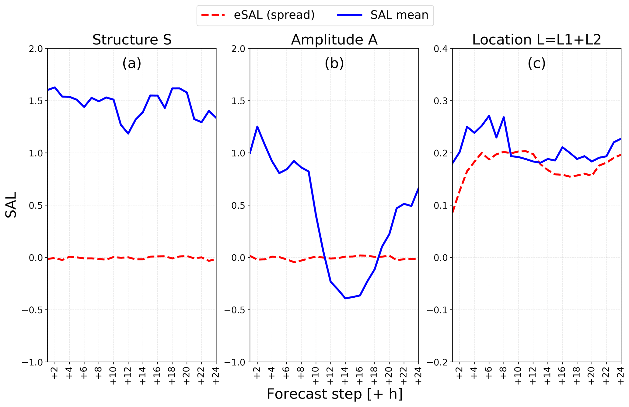
Figure 4(a) Structure, (b) amplitude and (c) location components of SAL for 24 forecast steps for the ensemble mean. The eSAL (or spread) has been calculated between all ensemble members.
The three components of the SAL analysis are shown in Fig. 4 for eSAL and the ensemble mean. The most evident result is that the eSAL (red dashed line) remains close to zero for the S and A components, meaning that the ensemble is not dispersive at all. This is somehow expected, as Structure and Amplitude describe the shape and magnitude of the lightning activity. Both components are dependent on the LPI algorithm itself or on how the model generally processes convection – how strong and how sparse – with all the members finally looking very similar. Therefore, when averaging over large datasets, the random discrepancies between the ensemble members get filtered out. The Location component is different, as it is more easily influenced by – and very sensitive to – perturbation of the model physics. However, given that the eSAL method has been thoroughly tested only for precipitation fields so far, there is also the possibility that the Structure and Amplitude components are not well defined quantities for probabilistic lightning verification. Nevertheless, a few comments can be made about the classical SAL analysis. According to the Structure plot, areas with lightning activity are in general too widespread and intense in the COSMO-D2 EPS compared to the observed activity. When looking at the Amplitude component for the ensemble mean (blue lines in Fig. 4), there is clearly an overestimation of the lightning activity especially during nighttime hours. This is in accordance with some preliminary statistical checks. In fact, by comparing the daily distribution of the two datasets relative to the daily maximum, the overestimation for this time window becomes evident.
The most interesting part of the SAL analysis is the Location component. In this case, the eSAL, which represents the spread of the system, is slightly lower compared to the classical SAL for the ensemble mean, representing the error. This means that the EPS is slightly underestimating the spatial uncertainty, which is consistent with the results from the eFSS/dFSS analysis. Both the SAL and the eSAL show a secondary minimum during the main convective window. This could be related to a more scattered signal when convection activity is low and a more predictable signal when it is organized (afternoon). The spread-error relationship is however slightly better compared to the FSS study. This likely relates to the fact that the Location component of the SAL is focusing only on the centers of mass of the fields, while letting the other two components take care of eventual bias in the magnitude or intensity of the fields. By comparing the two results, one possible conclusion is that the COSMO-D2 EPS performs well in terms of skill and spread-error relationship when it comes to spatial errors and uncertainties for lightning activity. Some concerns remain with respect to possible biases affecting both the overall magnitude of the fields and the shape/intensity of the single objects. Finally, the analysis of the single components L1 and L2 (not shown here) do not add much information to the study, with only negligible differences between the two.
Innovative verification methods have been applied to the high resolution COSMO-D2-EPS LPI in order to analyze the skill of the system and the ability of the ensemble to forecast the predictability of lightning activity. For the afternoon hours, an average skillful scale of 220 km has been determined for the summer months of 2019, while the EPS would rate the forecast as useful already at around 110 km. This means that the EPS is overall slightly underdispersive. In any case, the eFSS/dFSS comparison shows that the probabilistic approach can help smoothing specific issues such as the delayed triggering of the first convective cells in the model. The SAL method confirms the lack of spread between the ensemble members, but it highlights the fact that the system is fairly good at localizing the areas with lightning activity. Some concerns remain with respect to possible biases in magnitude and intensity of the forecast.
As this study was just a first attempt at addressing whether convective-scale ensembles can forecast lightning with any skill, there are several areas where this analysis can be developed further. First of all, other model runs such as the 03:00, 06:00, 09:00 or 12:00 UTC should also be added to the dataset in order to evaluate the role and importance of data assimilation in improving the skill during the afternoon hours, when most of the lightning strikes occur. This would also decouple the forecast steps from the hour of the day, leading to a much more significant analysis of the spread-error relationship as a function of the forecast lead time.
Furthermore, in this study the datasets have been analyzed on an hourly frequency, but potentially a much more detailed analysis is possible with the COSMO-D2 fields being available every 15 min. This might help locating the issue regarding the delayed triggering of the diurnal convective cycle with a higher temporal precision. However, an increase in the temporal resolution often leads to lower skill for lightning forecasts (Mittermaier et al., 2022a, b). Another aspect which might be investigated is the different skill and spread-error relationship between different geographical and topographical regions. For example, the model performance in forecasting deep convection in the alpine region might be considerably better compared to the lowlands in Central Europe. Other areas that could be investigated include the comparison between the LPI and other convective indices (both based on parcel theory and cloud microphysics) in a high resolution EPS or the usage of other non-conventional observational datasets in addition to lightning strikes, such as satellite pattern recognition applied to convective cells.
The real time forecast products of the new ICON-D2 EPS (which has replaced the COSMO-D2 EPS at the DWD as operational convection-permitting ensemble) are freely available on the Opendata portal of the German Weather Service and also include the Lightning Potential Index (https://opendata.dwd.de/weather/nwp/icon-d2-eps/; Deutscher Wetterdienst, 2022). The original COSMO-D2 EPS and LINET datasets for the Summer 2019 used in this work as well as all the Python scripts are also available upon request by email (Michele Salmi – a01656041@unet.univie.ac.at).
CM and MS designed the study. MS ran the simulations, made the plots, performed the analysis and wrote the manuscript. MD provided important guidance, while all the authors discussed and revised the manuscript.
The contact author has declared that neither they nor their co-authors have any competing interests.
Publisher's note: Copernicus Publications remains neutral with regard to jurisdictional claims in published maps and institutional affiliations.
This article is part of the special issue “21st EMS Annual Meeting – virtual: European Conference for Applied Meteorology and Climatology 2021”.
The authors appreciate the inspiring insights provided by several researchers at Meteoschweiz/Meteosuisse, who are also conducting research on the LPI at very high horizontal resolutions.
This paper was edited by Daniel Reinert and reviewed by Marion Mittermaier and one anonymous referee.
Baldauf, M., Gebhardt, C., Theis, S., Ritter, B., and Schraff, C.: Beschreibung des operationellen Kürzestfristvorhersagemodells COSMO-D2 und COSMO-D2-EPS und seiner Ausgabe in die Datenbanken des Deutscher Wetterdienstes (DWD), Technical Report, https://www.dwd.de/DE/leistungen/nwv_cosmo_d2_aenderungen/nwv_cosmo_d2_aenderungen.html (last access: 28 May 2022), 2018. a
Betz, H.-D., Schmidt, K., Oettinger, P., Wirz, M.: Lightning detection with 3-D discrimination of intracloud and cloud-to-ground discharges, Geophys. Res. Lett., 31, L11108, https://doi.org/10.1029/2004GL019821, 2004. a
Betz, H.-D., Schmidt, K., Laroche, P., Blanchet, B., Oettinger, W. P., Defer, E., Dziewit, Z., and Konarski, J.: LINET-An international lightning detection network in Europe, Atmos. Res., 91, 564–573, https://doi.org/10.1016/j.atmosres.2008.06.012, 2009. a
Blahak, U.: LPI (Lightning Potential Index) derived from COSMO-DE fields, COSMO General Meeting Wroclaw 2015, https://www.cosmo-model.org/content/consortium/generalMeetings/general2015/parallel/lpi_blahak.pdf (last access: 28 May 2022), 2015. a, b
Deutscher Wetterdienst: Open Data Server of the German Meteorological Service (DWD), Deutscher Wetterdienst [data set], https://opendata.dwd.de/weather/nwp/icon-d2-eps/, last access: 28 May 2022. a
Dey, S. R. A., Leoncini, G., Roberts, N. M., Plant, R. S., and Migliorini, S.: A spatial view of ensemble spread in convection permitting ensembles, Mon. Weather Rev., 142, 4091–4107, https://doi.org/10.1175/MWR-D-14-00172.1, 2014. a, b
Faggian, N., Roux, B., Steinle, P., and Ebert, B.: Fast calculation of the fractions skill score, Mausam, 66, 457–466, https://doi.org/10.54302/mausam.v66i3, 2015. a
Ferro, C. A. T. and Stephenson, D. B.: Extremal dependence indices: improved verification measures for deterministic forecasts of rare binary events, Weather Forecast., 26, 699–713, https://doi.org/10.1175/WAF-D-10-05030.1, 2011. a
Gebhardt, C., Theis, S. E., Paulat, M., and Ben Bouallègue, Z.: Uncertainties in COSMO-DE precipitation forecasts introduced by model perturbations and variation of lateral boundaries, Atmos. Res., 100, 168–177, https://doi.org/10.1016/j.atmosres.2010.12.008, 2011. a
Karagiannidis, A., Lagouvardos, K., Lykoudis, S., Kotroni, V., Giannaros, T., and Betz, H. D.: Modeling lightning density using cloud top parameters, Atmos. Res., 222, 163–171, https://doi.org/10.1016/j.atmosres.2019.02.013, 2019. a
LeDuc, K. S. and Hiromu, S.: Spatial-temporal fractions verification for high-resolution ensemble forecasts, Tellus A, 65, 18171, https://doi.org/10.3402/tellusa.v65i0.18171, 2013. a
Lynn, B. and Yair, Y.: Prediction of lightning flash density with the WRF model, Adv. Geosci., 23, 11–16, https://doi.org/10.5194/adgeo-23-11-2010, 2010. a, b
Lynn, B. H., Yair, Y., Price, C., Kelman, G., and Clark, A. J.: Predicting cloud-to-ground and intracloud lightning in weather forecast models, Weather Forecast., 27, 1470–1488, https://doi.org/10.1175/WAF-D-11-00144.1, 2012. a, b
Marsigli, C., Alferov, D., Astakhova, E., Duniec, G., Gayfulin, D., Gebhardt, C., Interewicz, W., Loglisci, N., Marcucci, F., Mazur, A., Montani, A., Tsyrulnikov, M., and Walser, A.: Studying Perturbations for the Representation of modeling uncertainties in Ensemble Development (SPRED Final Report), COSMO Technical Report, 39, https://www.cosmo-model.org/content/model/documentation/techReports/cosmo/docs/techReport39.pdf (last access: 28 May 2022), 2019. a
McCaul, E. W., Goodman, S. J., LaCasse, K. M., and Cecil, D. J.: Forecasting Lightning Threat Using Cloud-Resolving Model Simulations, Weather Forecast., 24, 709–729, https://doi.org/10.1175/2008WAF2222152.1, 2009. a, b
Mittermaier, M. P.: A “Meta” Analysis of the Fractions Skill Score: The Limiting Case and Implications for Aggregation, Mon. Weather Rev., 149, 3491–3504, https://doi.org/10.1175/MWR-D-18-0106.1, 2021. a
Mittermaier, M., Wilkinson, J., Csima, G., Goodman, S., and Virts, K.: Convective-scale numerical weather prediction and warnings over Lake Victoria: Part I – Evaluating a lightning diagnostic, Meteorol. Appl., 29, e2038, https://doi.org/10.1002/met.2038, 2022a. a
Mittermaier, M., Landman, S., Csima, G., and Goodman, S.: Convective-scale numerical weather prediction and warnings over Lake Victoria, Part II: Can model output support severe weather warning decision-making?, Meteorol. Appl., 29, e2055, https://doi.org/10.1002/met.2055, 2022b. a
Montani, A., Capaldo, M., Cesari, D., Marsigli, C., Modigliani, U., Nerozzi, F., Paccagnella, T., and Tibaldi, S.: Operational limited – area ensemble forecasts based on the `Lokal Modell', ECMWF Newsletter, 98, 2–7, https://www.ecmwf.int/sites/default/files/elibrary/2003/14626-newsletter-no98-summer-2003.pdf (last access: 28 May 2022), 2003. a
Radanovics, S., Vidal, J.-P., and Sauquet, E.: Spatial verification of ensemble precipitation: an ensemble version of SAL, Weather Forecast., 33, 1001–1020, https://doi.org/10.1175/WAF-D-17-0162.1, 2018. a, b, c
Reinert, D., Prill, F., Frank, H., Denhard, M., Baldauf, M., Schraff, C., Gebhardt, C., Marsigli, C., and Zängl, G.: DWD Database Reference for the Global and Regional ICON and ICON-EPS Forecasting System, DWD, https://www.dwd.de/DWD/forschung/nwv/fepub/icon_database_main.pdf (last access: 28 May 2022), 2021. a
Roberts, N. and Lean, H.: Scale-selective verification of rainfall accumulations from high-resolution forecasts of convective events, Mon. Weather Rev., 136, 78–97, https://doi.org/10.1175/2007mwr2123.1, 2008. a, b, c
Rossa, A. M., Nurmi, P., and Ebert, E. E.: Precipitation: Advances in Measurement, Estimation and Prediction, Springer, 418–450, ISBN 978-3-540-77654-3, e-ISBN 978-3-540-77655-0, 2008. a
Saunders, C. P. R.: Charge separation mechanisms in clouds, Space Sci. Rev., 137, 335–354, https://doi.org/10.1007/978-0-387-87664-1_22, 2008. a
Schraff, C., Reich, H., Rhodin, A., Schomburg, A., Stephan, K., Periáñez, A., and Potthast, R.: Kilometre-scale ensemble data assimilation for the COSMO model (KENDA), Q. J. Roy. Meteorol. Soc., 142, 1453–1472, https://doi.org/10.1002/qj.2748, 2016. a
Wernli, H., Paulat, M., Hagen, M., and Frei, C.: SAL-A novel quality measure for the verification of quantitative precipitation forecasts, Mon. Weather Rev., 136, 4470–4487, https://doi.org/10.1175/2008MWR2415.1, 2008. a, b, c